Model, Evaluate, and Design Acoustic Spaces
In this example, you model, analyze, and optimize the acoustics of an indoor space. You will:
Define a room with sources and receivers
Estimate reverberation time (RT-60) using analytical and physical models
Simulate room impulse responses using the
acousticRoomResponsefunctionEvaluate acoustics using standard-based metrics RT-60 and speech transmission index (STI) with the
rt60andspeechTransmissionIndexfunctionsEvaluate the room acoustics and scenario effects on speech using the popular metrics short-time objective intelligibility (STOI) and virtual speech and quality objective listener (ViSQOL) with the
stoiandvisqolfunctionsAnalyze the effects of source, noise, and listener positions on acoustics and speech transmission
Choose a material to optimize an acoustic metric
The workflow is applicable to classrooms, lecture halls, studios, and other indoor spaces.
Define and Visualize Room
Use the supporting function iGetClassroom to return a struct array containing the dimensions, surface material coefficients, and locations for a source, receiver, and noise source. Dimensions and locations are given in meters. The center frequencies are given in hertz.
room = iGetClassroom()
room = struct with fields:
             Dimensions: [14 12 5]
      CenterFrequencies: [125 250 500 1000 2000 4000]
     MaterialAbsorption: [6×6 double]
     MaterialScattering: [6×6 double]
         SourceLocation: [2 6 2]
       ReceiverLocation: [12 6 1.5000]
    NoiseSourceLocation: [7.3000 5.3000 3.9000]
            Description: "Empty Classroom"
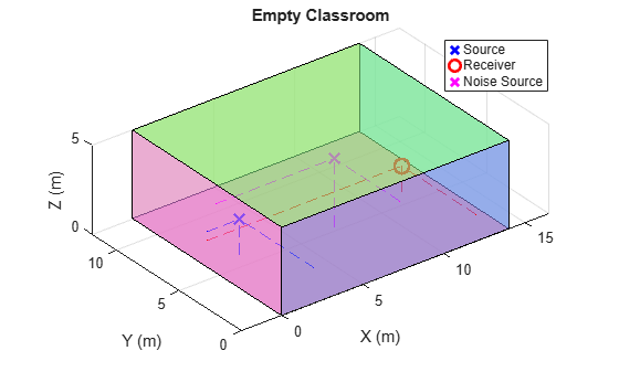
Use the supporting function iPlotRoom to visualize. An empty rectangular room, as shown here, is called a "shoe-box" model and can be used for some gross analysis and pedagogy. A more realistic analysis would include models of furniture and occupants.
iPlotRoom(room)
Estimate RT-60 Using Sabine's Formula
The Sabine equation estimates the reverberation time (RT-60), which is the time it takes for sound to decay 60 decibels after the source stops. Published by Wallace Clement Sabine in 1900, it is the first reverberation-time equation and continues to be a fundamental tool of architectural acoustics [1]. The formula relates the reverberation time with a room's volume and absorption:
,
where is the reverberation time in seconds, is the room volume in , and is the total absorption of the room in metric sabins. The total absorption is computed as the sum of the surface areas multiplied by their respective absorption coefficients, .
Material absorption coefficients vary with frequency, so RT-60 values are frequency-dependent:
.
The Sabine equation does not account for the source/receiver positions, scattering or air absorption; it is a general formula best for rooms with average absorption coefficients below 0.25.
Use the supporting function iRT60model to estimate the frequency-dependent RT-60.
t60 = iRT60model(room)
t60=1×6 table
      125       250      500      1000      2000      4000
    _______    ______    ____    ______    ______    ______

    0.85087    1.2645    1.68    1.5737    1.3832    1.4895
Simulate Room Impulse Response
To analyze a room with a more complex physical model, use acousticRoomResponse to estimate an impulse response based on dimensions, materials, and source/receiver locations. The function supports the image-source, stochastic ray tracing, and hybrid methods. For image-source modeling, estimate the required order (number of reflections) by:
,
where
is the image source order
is the speed of sound
is the frequency-dependent RT-60
is the volume
is the surface area
The quantity is sometimes called the mean free path and is the average distance a sound travels between two successive reflections. The quantity represents the total distance traveled to achieve the frequency-dependent RT-60.
Use the supporting function iEstimateImageSourceOrder to estimate the image source order required to achieve the estimated RT-60 value.
imageSourceOrder = iEstimateImageSourceOrder(room,t60)
imageSourceOrder =
29
Use the acousticRoomResponse function to model the room's impulse response. Use the order derived analytically to set the ImageSourceOrder. The NumStochasticRays and MaxNumRayReflections parameters were chosen empirically to balance speed and accuracy.
fs = 16e3; % Sample rate
rirt = acousticRoomResponse(room.Dimensions,room.SourceLocation,room.ReceiverLocation, ...
    BandCenterFrequencies=room.CenterFrequencies, ...
    MaterialAbsorption=room.MaterialAbsorption, ...
    MaterialScattering=room.MaterialScattering, ...
    ImageSourceOrder=imageSourceOrder, ...
    NumStochasticRays=5120, ...
    MaxNumRayReflections=40, ...
    SampleRate=fs);
The acousticRoomResponse function returns an idealized room impulse response. Use the supporting function iAddNoiseFloor to add a noise floor to better simulate a real measurement. A -60 dB noise floor provides enough range for the impulse response for accurate RT-60 estimations.
noiseFloor = -60;
rir = iAddNoiseFloor(rirt,fs,noiseFloor);
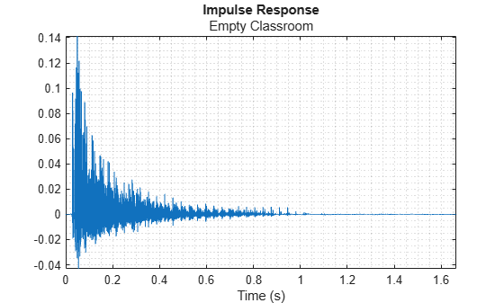
Visualize the impulse response.
tvec = (0:numel(rir)-1)/fs;

figure
plot(tvec,rir)
xlabel("Time (s)")
axis tight
title("Impulse Response",room.Description)
grid minor
Evaluate Acoustic Metrics
Audio Toolbox™ provides the rt60 function and the speechTransmissionIndex function to evaluate acoustic spaces. RT-60 characterizes the suitability of a space as a listening environment for various uses, such as concert venues and lecture halls. Speech transmission index is a measurement of a room's ability to transmit intelligible speech. It is used to analyze and improve the intelligibility of an acoustic space and is often a required metric of regulatory bodies, especially in cases where public address systems are present.
Reverberation Time (RT-60)
Use the rt60 function to calculate the RT-60 value according to the ISO 3382-1 standard. The function returns a table listing the frequency-dependent reverberation time as well as additional metrics described in the standard such as the early decay time, clarity and definition. T20, T30, and Topt represent measurements of the reverberation time. T20 is the time it takes for the impulse response energy to decay 20 dB after an initial decay of 5 dB which represents the early reflections. T30 is the time it takes the impulse response energy to decay 30 dB after the initial decay. Topt represents an RT-60 estimate by choosing the part of the energy decay curve that provides the best linear fit and then extrapolating the RT-60 value from that. For more details on the algorithm and metric interpretation, see rt60 and [2]. Note that for real standard-compliant measurements, there are requirements on the source and receiver locations detailed in [2].
The RT-60 values calculated here are considerably different than the RT-60 values predicted by the Sabine equation. This is because the RT-60 values given by the Sabine equation represent a rough and simplistic approximation. The equation was derived empirically and does not account for positions in the room, frequency dependency except through absorption coefficients, or scattering coefficients. The acousticRoomResponse physical modeling is also a rough approximation, although it can be improved by modeling the room with a triangulation object providing more specific material coefficients, as well as by increasing the image-source order and the number of stochastic rays and reflections.
t60comp = rt60(rir,fs)
t60comp=6×11 table
    CenterFrequencies     EDT       T20       T30       Topt             DegreeOfNonLinearity            Curvature      C50         C80       D50         Ts
    _________________    ______    ______    ______    ______    ____________________________________    _________    ________    _______    ______    ________

           125           2.5684    2.8531       NaN    2.9292    27.583    9.5841    5.3501    5.3501         NaN      -1.8343    0.55159    39.595     0.17044
           250           2.9076    2.5313       NaN    3.3409    47.982    44.915    28.507    8.1426         NaN      -1.4063    0.12663    41.975     0.15497
           500           2.1905    2.4163    1.9414    3.1281    12.685    37.857    27.263    6.8863     -19.655      -2.9861    -1.3775    33.457     0.15339
          1000           1.8686    1.8507    1.6648    2.1484    18.234    6.1402    10.673    3.9593     -10.044     -0.82179     1.1641    45.283     0.11692
          2000           1.2663     2.068    1.9292    2.0508    13.354    4.6018    10.879    3.6828     -6.7125     -0.42624     1.8723    47.548     0.09133
          4000           1.2011    1.6401    1.6331    1.3041    5.3573    10.971    6.5354     1.806    -0.42662     -0.60737     1.9534    46.509    0.086709
Call the rt60 function a second time without any input arguments to visualize the frequency-dependent RT-60 and inspect the energy decay and best fit lines for individual octave bands. You can use this view to inspect the energy decay curve (EDC) and the fit of T20, T30, and Topt. It is a good diagnostic tool for verifying measurements and identifying potential sources of error in your measurement.
figure
rt60(rir,fs)
![Figure contains 2 axes objects. Axes object 1 with title RT-60, xlabel Octave Center Frequency (Hz), ylabel Time (s) contains 9 objects of type stair, line, patch. One or more of the lines displays its values using only markers These objects represent EDT, T20, T30, Topt. Axes object 2 with title Octave Center Frequency - 1000 Hz, xlabel Time (s), ylabel dB contains 6 objects of type line. These objects represent IR, EDC, EDT [0,-10] : 1.869 s, T20 [-5,-25] : 1.851 s, T30 [-5,-35] : 1.665 s, Topt [-5,-15] : 2.148 s.](../../examples/audio/win64/ModelEvaluateAndDesignAcousticSpacesExample_03.png)
Speech Transmission Index (STI)
Call the speechTransmissionIndex function to characterize the room's ability to transmit intelligible speech according to IEC 60268-16:2020. The speech transmission index is a scalar in the interval [0,1]. As the value increases from 0 to 1, the quality of speech transmission index increases. An STI value of 0.46 is considered the lower limit for voice alarm systems. For details on the algorithm and metric interpretation, see speechTransmissionIndex and [3].
When speechTransmissionIndex is called with no additional arguments, the room impulse response (RIR) is assumed to be a high SNR capture and is calculated with values suggested by the standard for the operational signal and noise levels.
stiMetric = speechTransmissionIndex(rir,fs)
stiMetric =
0.5022
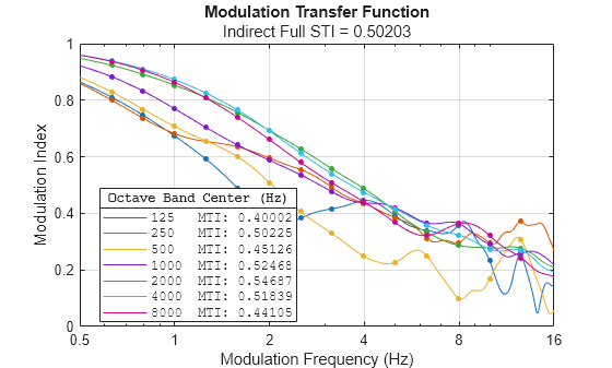
Call speechTransmissionIndex a second time without any output arguments to visualize the modulation transfer function as well. The speech transmission index algorithm uses the modulation transfer function (MTF) as an intermediate representation before deriving the STI. Analyzing the MTF provides insight into the causes of poor speech intelligibility. For example, if the MTF is relatively flat, low speech intelligibility is mainly determined by background noise. A continuously decreasing MTF indicates the influence of reverberation.
figure
speechTransmissionIndex(rir,fs)
Evaluate Speech Metrics
Audio Toolbox™ provides the stoi and visqol functions to evaluate speech transmission using a referenced (source) and degraded (receiver) pair. These functions are agnostic to how the speech was processed and are often used for the evaluation of communication systems and speech enhancement systems.
Model a prototypical speech signal at the receiver by convolving with the RIR. The subsequent metrics are level-independent so there is no need to account for level differences at the source and receiver.
[speech,xfs] = audioread("CleanSpeech-16-mono-3secs.ogg");
speech = audioresample(mean(speech,2),InputRate=xfs,OutputRate=fs);

receivedSpeech = fftfilt(rir,speech);
Short-Time Object Intelligibility (STOI)
Call the stoi function specifying the received and transmitted speech to view the effect of the acoustic space on speech intelligibility. The STOI metric is a scalar in the range [-1,1]. A higher value for the metric corresponds to a more intelligible speech signal.
stoiMetric = stoi(receivedSpeech,speech,fs)
stoiMetric =
0.2709
Virtual Speech Quality Objective Listener (ViSQOL)
Call the visqol function specifying the received and transmitted speech to view the effect of the acoustic space on speech intelligibility. The default ViSQOL metric represents the mean opinion score (MOS) and is a scalar in the range [1,5], where a higher value corresponds to higher quality.
visqolMetric = visqol(receivedSpeech,speech,fs,Mode="speech")visqolMetric = 2.3492
Analyze Effect of Noise Source
In this section, you add a noise source to your acoustic model.
Re-estimate the image-source order required to model the impulse response. Use the reverberation time derived from the acousticRoomResponse and rt60 functions.
imageSourceOrder = iEstimateImageSourceOrder(room,t60comp.Topt)
imageSourceOrder =
58
Use the acousticRoomResponse function to model the room's impulse response given a noise source location. Add a noise floor to the simulated measurement.
noiseRIR = acousticRoomResponse(room.Dimensions,room.NoiseSourceLocation,room.ReceiverLocation, ...
    BandCenterFrequencies=room.CenterFrequencies, ...
    MaterialAbsorption=room.MaterialAbsorption, ...
    MaterialScattering=room.MaterialScattering, ...
    ImageSourceOrder=imageSourceOrder, ...
    NumStochasticRays=5120, ...
    MaxNumRayReflections=40, ...
    SampleRate=fs);
noiseRIR = iAddNoiseFloor(noiseRIR,fs,noiseFloor);
Model a prototypical noise signal at the receiver by convolving with the RIR.
[noise,xfs] = audioread("WashingMachine-16-44p1-stereo-10secs.wav");
noise = audioresample(mean(noise,2),InputRate=xfs,OutputRate=fs);
noise = resize(noise,size(receivedSpeech),Side="both");

receivedNoise = fftfilt(noiseRIR(:),noise);
Model the speech signal at the source as having an overall sound pressure level (SPL) of 62.35 dB.
levelatsource = 62.35;
Calculate the speech signal at the receiver using a common dB energy decay approximation.
distance = norm(room.ReceiverLocation - room.SourceLocation);
levelatreceiver = levelatsource - 20*log10(distance);
Scale the source speech signal to the target receiver levels.
scaleAudio = @(x,targetSPL) x * ((20e-6 * 10^(targetSPL/20)) / rms(x));
receivedSpeechScaled = scaleAudio(receivedSpeech,levelatreceiver);
Model the noise signal as having an overall SPL level of 50 dB.
noiselevelatsource = 50;
Calculate the noise signal at the receiver using a common dB energy decay approximation.
noisedistance = norm(room.ReceiverLocation - room.NoiseSourceLocation);
noiselevelatreceiver = noiselevelatsource - 20*log10(noisedistance);
Scale the source noise signal to the target receiver levels.
receivedNoiseScaled = scaleAudio(receivedNoise,noiselevelatreceiver);
Determine the octave SPL of the received speech and noise signals. Use the splMeter function to measure the equivalent continuous SPL for the entire time interval.
SPL = splMeter( ...
    Bandwidth="1 octave", ...
    FrequencyRange=[100,8500], ...
    FrequencyWeighting="A-weighting", ...
    OctaveFilterOrder=56, ...
    TimeInterval=fs/numel(speech), ...
    SampleRate=fs);
[~,Leq] = SPL(receivedSpeechScaled);
speechLevels = Leq(end,:);
reset(SPL)
[~,Leq] = SPL(receivedNoiseScaled);
noiseLevels = Leq(end,:);

OctaveSPL = array2table([speechLevels;noiseLevels], ...
RowNames=["Speech (dB)", "Noise (dB)"], ...
VariableNames=["125","250","500","1000","2000","4000","8000"])
OctaveSPL=2×7 table
                    125       250       500       1000      2000       4000       8000
                   ______    ______    ______    ______    ______    ________    _______

    Speech (dB)    15.199    20.665    30.648    32.946    22.968      7.2816    -1.6141
    Noise (dB)     4.6088     7.598     14.06    14.155    6.3777    -0.95794    -23.848
Evaluate Acoustic Metrics with Noise Source
The rt60 metric is independent of any noise sources. The associated measurements should be made under noiseless conditions.
The speechTransmissionIndex metric does account for noise sources. When measuring STI directly under noisy conditions, you can remove the effect of noise and add operational noise using RemoveRawAmbientNoise and AddOperationalAmbientNoise, respectively. When calculating STI using the indirect method, the RIR is assumed to be captured under noiseless conditions and you can set expected noise and signal levels by specifying OperationalNoiseLevel and OperationalSignalLevel. By default, AddOperationalAmbientNoise is set to true.
Speech Transmission Index (STI) with Noise
Calculate the speech transmission index for the scenario by specifying the operational signal and noise levels.
stiMetric_noisePresent = speechTransmissionIndex(rir,fs, ...
    OperationalNoiseLevel=noiseLevels, ...
    OperationalSignalLevel=speechLevels);
fprintf('STI: %.2f\nSTI with Noise Source: %.2f\n',stiMetric,stiMetric_noisePresent);
STI: 0.50
STI with Noise Source: 0.41
Evaluate Speech Metrics with Noise Source
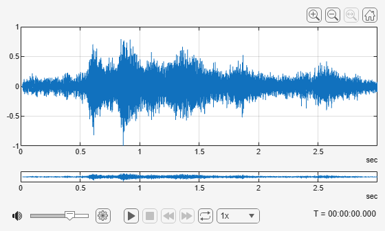
Model the received signal by combining the speech and noise. Use Audio Viewer to plot and listen to the transmitted speech and the received speech.
receivedNoisySpeech = receivedSpeechScaled + receivedNoiseScaled;
audioViewer(speech./max(abs(speech)),fs)
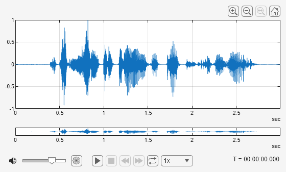
audioViewer(receivedNoisySpeech./max(abs(receivedNoisySpeech)),fs)
Short-Time Object Intelligibility (STOI) with Noise Source
Call the stoi function specifying the received and transmitted speech to view the effect of the acoustic space with noise on speech intelligibility. Compare the metrics before and after modeling the noise source. The STOI metric improves under the low-level noise.
stoiMetric_noisePresent = stoi(receivedNoisySpeech,speech,fs);
fprintf('STOI: %.2f\nSTOI with Noise Source: %.2f\n',stoiMetric,stoiMetric_noisePresent);
STOI: 0.27 STOI with Noise Source: 0.30
Virtual Speech Quality Objective Listener (ViSQOL) with Noise Source
Call the visqol function specifying the received and transmitted speech to view the effect of the acoustic space on speech intelligibility. Compare the metrics before and after modeling the noise source.
visqolMetric_noisePresent = visqol(receivedNoisySpeech,speech,fs,Mode="speech");
fprintf('ViSQOL: %.2f\nViSQOL with Noise Source: %.2f\n',visqolMetric,visqolMetric_noisePresent);
ViSQOL: 2.35
ViSQOL with Noise Source: 1.81
Analyze Effect of Listener Position
In this next section, you build upon the previous model by moving the listener position and recording the resulting STI, STOI, and ViSQOL.
Model Received Signal at Variable Position
Create a grid of the X-Y (floor) plane of the room. Vary the listener (receiver) location. Reduce the image-source order and number of stochastic rays to complete this parameter sweep in a reasonable amount of time. If you have Parallel Computing Toolbox™, the parameter sweep takes place using your default pool configuration.
numxtiles = 10;
numytiles = 9;
xlocs = linspace(0,room.Dimensions(1),numxtiles);
ylocs = linspace(0,room.Dimensions(2),numytiles);
stoiloc = nan(numxtiles,numytiles);
visqolloc = nan(numxtiles,numytiles);
stiloc = nan(numxtiles,numytiles);

parfor xlocidx = 1:numxtiles
    for ylocidx = 1:numytiles
        receiverLocation = [xlocs(xlocidx),ylocs(ylocidx),room.Dimensions(3)];
        rirAtLoc = acousticRoomResponse(room.Dimensions,room.SourceLocation,receiverLocation, ...
            BandCenterFrequencies=room.CenterFrequencies, ...
            MaterialAbsorption=room.MaterialAbsorption, ...
            MaterialScattering=room.MaterialScattering, ...
            ImageSourceOrder=30, ...
            NumStochasticRays=2048, ...
            MaxNumRayReflections=20, ...
            SampleRate=fs);
        rirAtLoc = iAddNoiseFloor(rirAtLoc,fs,noiseFloor);
        noiseRIRatLoc = acousticRoomResponse(room.Dimensions,room.NoiseSourceLocation,receiverLocation, ...
            BandCenterFrequencies=room.CenterFrequencies, ...
            MaterialAbsorption=room.MaterialAbsorption, ...
            MaterialScattering=room.MaterialScattering, ...
            ImageSourceOrder=30, ...
            NumStochasticRays=2048, ...
            MaxNumRayReflections=20, ...
            SampleRate=fs);
        noiseRIRatLoc = iAddNoiseFloor(noiseRIRatLoc,fs,noiseFloor);

        receivedSpeechScaled = fftfilt(rirAtLoc,speech);
        receivedNoiseScaled = fftfilt(noiseRIR,noise);

        speechTotalLevel = levelatsource - 20*log(norm(room.SourceLocation - receiverLocation));
        noiseTotalLevel = noiselevelatsource - 20*log(norm(room.NoiseSourceLocation - receiverLocation));

        receivedSpeechScaled = scaleAudio(receivedSpeechScaled,speechTotalLevel);
        receivedNoiseScaled = scaleAudio(receivedNoiseScaled,noiseTotalLevel);

        receivedNoisySpeech = receivedSpeechScaled + receivedNoiseScaled;

        stoiloc(xlocidx,ylocidx) = stoi(receivedNoisySpeech,speech,fs);
        visqolloc(xlocidx,ylocidx) = visqol(receivedNoisySpeech,speech,fs);

        reset(SPL)
        [~,Leq] = SPL(receivedNoiseScaled);
        noiseLevels = Leq(end,:);

        reset(SPL)
        [~,Leq] = SPL(receivedSpeechScaled);
        speechLevels = Leq(end,:);

        stiloc(xlocidx,ylocidx) = speechTransmissionIndex(rirAtLoc,fs, ...
            OperationalNoiseLevel=noiseLevels, ...
            OperationalSignalLevel=speechLevels);
    end
end
Visualize Effect of Listener Position on Metrics
Use the supporting function iPlotMetricSweep to display how the STI, STOI, and ViSQOL metrics vary with the receiver position. As expected, all metrics increase as the receiver gets close to the source and decrease as the receiver gets close to the noise source.
iPlotMetricSweep(xlocs,ylocs,stiloc,room,"STI")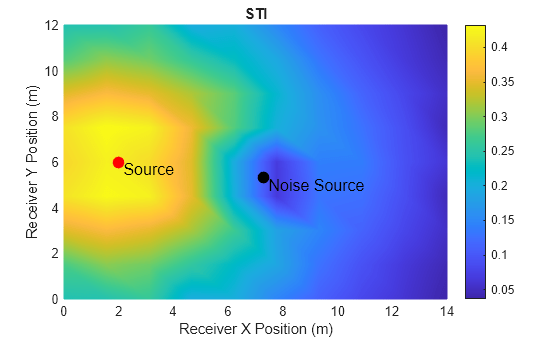
iPlotMetricSweep(xlocs,ylocs,stoiloc,room,"STOI")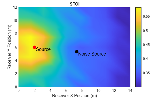
iPlotMetricSweep(xlocs,ylocs,visqolloc,room,"ViSQOL")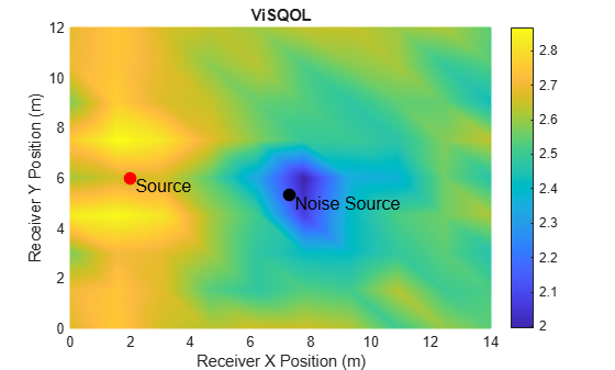
Select Surface Material for Metric Optimization
In this section, you evaluate different ceiling materials for their effect on the STI.
Define some material absorption coefficients. Each material has octave-band absorption coefficients (125 Hz to 4 kHz). These coefficients are given in [1]. Scattering coefficients are less readily available. For simplicity, use the same scattering coefficients for all materials.
materialChoices = {"Acoustical Tile, ave, 1/2-in thick",[0.07,0.21,0.66,0.75,0.62,0.49]; ...
    "Acoustical Tile, ave, 3/4-in thick",[0.09,0.28,0.78,0.84,0.73,0.64]; ...
    "Owens-Corning Frescor: painted, 5/8-in thick, mounting 7",[0.69,0.86,0.68,0.87,0.90,0.81]; ...
    "Gypsum board: 1/2-in",[0.29,0.10,0.05,0.04,0.07,0.09]};
Model the room impulse response for each material and record the resulting speech transmission index.
stiCeilingMaterial = zeros(size(materialChoices,1),1);
for ii = 1:size(materialChoices,1)
    roomAbsorption = [room.MaterialAbsorption(1:5,:);materialChoices{ii,2}];
    rir = acousticRoomResponse(room.Dimensions,room.SourceLocation,room.ReceiverLocation, ...
        BandCenterFrequencies=room.CenterFrequencies, ...
        MaterialAbsorption=roomAbsorption, ...
        MaterialScattering=room.MaterialScattering, ...
        ImageSourceOrder=imageSourceOrder, ...
        NumStochasticRays=5120, ...
        MaxNumRayReflections=40, ...
        SampleRate=fs);
    rir = iAddNoiseFloor(rir,fs,noiseFloor);
    stiCeilingMaterial(ii) = speechTransmissionIndex(rir,fs);
end
Display the STI for each ceiling material and the STI category and interpretation. Use the supporting function iGetQualificationBand to retrieve the STI category and interpretation defined in the IEC 60268-16 standard.
[band,type,example,comment] = iGetQualificationBand(stiCeilingMaterial);
T = table( ...
    string(materialChoices(:,1)), ...
    stiCeilingMaterial, ...
    string(band), ...
    string(type), ...
    string(example), ...
    string(comment), ...
    VariableNames=["Ceiling Material","STI","Category","Type of Message Information","Typical Uses","Comment"]);
T = sortrows(T,"STI","descend");
disp(T)
                         Ceiling Material                           STI      Category        Type of Message Information                                           Typical Uses                                                 Comment
    __________________________________________________________    _______    ________    ____________________________________    ________________________________________________________________________________    _____________________________

    "Owens-Corning Frescor: painted, 5/8-in thick, mounting 7"    0.52496      "F"       "complex messages, familiar context"    "PA systems in shopping malls, public buildings offices, VA systems, cathedrals"    "good quality PA systems"
    "Acoustical Tile, ave, 3/4-in thick"                           0.5159      "G"       "complex messages, familiar context"    "shopping malls, public buildings offices, VA systems"                              "target value for VA systems"
    "Acoustical Tile, ave, 1/2-in thick"                          0.50979      "G"       "complex messages, familiar context"    "shopping malls, public buildings offices, VA systems"                              "target value for VA systems"
    "Gypsum board: 1/2-in"                                        0.41712      "I"       "simple messages, familiar context"     "VA and PA systems in very difficult acoustic environments"                         "limited intelligibility"
Supporting Functions
Get Qualification Band
function [band, type, example, comment] = iGetQualificationBand(STI)
% Returns qualification banding for each STI value in vector
% Based on Annex G of IEC 60268-16:2020

n = numel(STI);
band = cell(n,1);
type = cell(n,1);
example = cell(n,1);
comment = cell(n,1);

for k = 1:n
    s = STI(k);
    if s < 0.36
        band{k}    = "U";
        type{k}    = "";
        example{k} = "not suitable for PA systems";
        comment{k} = "";
    elseif s < 0.40
        band{k}    = "J";
        type{k}    = "";
        example{k} = "not suitable for PA systems";
        comment{k} = "";
    elseif s < 0.44
        band{k}    = "I";
        type{k}    = "simple messages, familiar context";
        example{k} = "VA and PA systems in very difficult acoustic environments";
        comment{k} = "limited intelligibility";
    elseif s < 0.48
        band{k}    = "H";
        type{k}    = "simple messages, familiar words";
        example{k} = "VA and PA systems in difficult acoustic environments";
        comment{k} = "normal lower limit for VA systems";
    elseif s < 0.52
        band{k}    = "G";
        type{k}    = "complex messages, familiar context";
        example{k} = "shopping malls, public buildings offices, VA systems";
        comment{k} = "target value for VA systems";
    elseif s < 0.56
        band{k}    = "F";
        type{k}    = "complex messages, familiar context";
        example{k} = "PA systems in shopping malls, public buildings offices, VA systems, cathedrals";
        comment{k} = "good quality PA systems";
    elseif s < 0.60
        band{k}    = "E";
        type{k}    = "complex messages, familiar context";
        example{k} = "concert halls, modern churches";
        comment{k} = "high quality PA systems";
    elseif s < 0.64
        band{k}    = "D";
        type{k}    = "complex messages, familiar words";
        example{k} = "lecture theatres, classrooms, concert halls";
        comment{k} = "good speech intelligibility";
    elseif s < 0.68
        band{k}    = "C";
        type{k}    = "complex messages, unfamiliar words";
        example{k} = "theaters, speech auditoria, parliaments, courts, teleconferencing";
        comment{k} = "high speech intelligibility";
    elseif s < 0.72
        band{k}    = "B";
        type{k}    = "complex messages, unfamiliar words";
        example{k} = "theaters, speech auditoria, parliaments, courts, assistive hearing systems (AHS)";
        comment{k} = "high speech intelligibility";
    elseif s < 0.76
        band{k}    = "A";
        type{k}    = "complex messages, unfamiliar words";
        example{k} = "theaters, speech auditoria, parliaments, courts, assistive hearing systems (AHS)";
        comment{k} = "high speech intelligibility";
    else
        band{k}    = "A+";
        type{k}    = "";
        example{k} = "recording studios";
        comment{k} = "excellent intelligibility but rarely achievable in most environments";
    end
end
end
Add Noise Floor
function ir = iAddNoiseFloor(ir,fs,noiseFloor)
% Minimum duration for IR captures for ISO 3382 compliance
flength = ceil(1.6*fs);

% Zero-pad IR to minimum length
if numel(ir) < flength
    ir = resize(ir(:),flength);
else
    ir = ir(:);
end

% Generate pink noise and normalize rms.
noise = pinknoise(numel(ir),1);
noise = noise./rms(noise);

% Scale pink noise to desired rms.
noise_rms = max(abs(ir(:))) * 10^(noiseFloor/20);
noise = noise*noise_rms;

ir = ir + noise;

end
RT-60 Model (Sabine)
function t60table = iRT60model(room,options)
arguments
    room
    options.SoundSpeed (1,1) = 343 % (m/s)
end

alpha = room.MaterialAbsorption;

Lx = room.Dimensions(1); % Length
Ly = room.Dimensions(2); % Width
Lz = room.Dimensions(3); % Height

% Floor/ceiling
Sxy = Lx*Ly;
Syx = Sxy;

% Front/back
Sxz = Lx*Lz;
Szx = Sxz;

% Left/right
Syz = Ly*Lz;
Szy = Syz;

S = [Sxy;Syx;Sxz;Szx;Syz;Szy];

% Total Volume
V = prod(room.Dimensions);

% Compute the frequency-dependent effective absorbing area of the room surfaces.
A = sum(S.*alpha,1);

% Apply formula
t60 = (55.25/options.SoundSpeed)*V./A;

t60table = array2table(t60,VariableNames=arrayfun(@num2str,room.CenterFrequencies,UniformOutput=false));

end
Estimate Max Image-Source Order
function maxOrder = iEstimateImageSourceOrder(room,t60,options)
arguments
    room
    t60
    options.SoundSpeed (1,1) double = 343
end
Lx = room.Dimensions(1); % Length
Ly = room.Dimensions(2); % Width
Lz = room.Dimensions(3); % Height

if istable(t60)
    t60 = table2array(t60);
end

% Floor/ceiling
Sxy = Lx*Ly;
Syx = Sxy;

% Front/back
Sxz = Lx*Lz;
Szx = Sxz;

% Left/right
Syz = Ly*Lz;
Szy = Syz;

S = [Sxy;Syx;Sxz;Szx;Syz;Szy];

% Total Volume
V = prod(room.Dimensions);

meanFreePath = 4*V./S;
maxOrder = ceil(max((options.SoundSpeed.*t60)./meanFreePath,[],"all"));
end
Plot Room
function iPlotRoom(room)
% PLOTROOM Plot room, transmitter, receiver, and noise source with colored faces and projection lines
figure()

roomDimensions = room.Dimensions;
receiverCoord = room.ReceiverLocation;
sourceCoord = room.SourceLocation;
noiseCoord = room.NoiseSourceLocation;

L = roomDimensions(1);
W = roomDimensions(2);
H = roomDimensions(3);

% Define vertices and faces
verts = [0 0 0; L 0 0; L W 0; 0 W 0; 0 0 H; L 0 H; L W H; 0 W H];
faces = [1 2 3 4;   % Bottom
    5 6 7 8;   % Top
    1 2 6 5;   % Front
    4 3 7 8;   % Back
    1 4 8 5;   % Left
    2 3 7 6];  % Right

% Colors for each face
faceColors = [0.9 0.5 0.5;  % Bottom
    0.5 0.9 0.5;  % Top
    0.5 0.5 0.9;  % Front
    0.9 0.9 0.5;  % Back
    0.9 0.5 0.9;  % Left
    0.5 0.9 0.9]; % Right

patch(Vertices=verts,Faces=faces, ...
    FaceColor="flat",FaceVertexCData=faceColors, ...
    FaceAlpha=0.6,EdgeColor="k")
hold on

% Plot source, receiver, and noise source
h1 = plot3(sourceCoord(1),sourceCoord(2),sourceCoord(3),"xb",MarkerSize=10,LineWidth=2);

h2 = plot3(receiverCoord(1),receiverCoord(2),receiverCoord(3),"or",MarkerSize=10,LineWidth=2);

h3 = plot3(noiseCoord(1),noiseCoord(2),noiseCoord(3),"xm",MarkerSize=10,LineWidth=2);

% Projection lines for source (blue)
plot3([sourceCoord(1),sourceCoord(1)], [sourceCoord(2),sourceCoord(2)], [0,sourceCoord(3)],"--b")
plot3([sourceCoord(1),sourceCoord(1)], [0,sourceCoord(2)], [sourceCoord(3),sourceCoord(3)],"--b")
plot3([0 sourceCoord(1)], [sourceCoord(2),sourceCoord(2)], [sourceCoord(3),sourceCoord(3)],"--b")

% Projection lines for receiver (red)
plot3([receiverCoord(1),receiverCoord(1)], [receiverCoord(2),receiverCoord(2)], [0,receiverCoord(3)],"--r")
plot3([receiverCoord(1),receiverCoord(1)], [0,receiverCoord(2)], [receiverCoord(3),receiverCoord(3)],"--r")
plot3([0 receiverCoord(1)], [receiverCoord(2),receiverCoord(2)], [receiverCoord(3),receiverCoord(3)],"--r")

% Projection lines for noise source (magenta)
plot3([noiseCoord(1),noiseCoord(1)], [noiseCoord(2),noiseCoord(2)], [0,noiseCoord(3)],"--m")
plot3([noiseCoord(1),noiseCoord(1)], [0,noiseCoord(2)], [noiseCoord(3),noiseCoord(3)],"--m")
plot3([0,noiseCoord(1)], [noiseCoord(2),noiseCoord(2)], [noiseCoord(3),noiseCoord(3)],"--m")

% Labels and view
xlabel("X (m)")
ylabel("Y (m)")
zlabel("Z (m)")
grid on
axis equal
title(room.Description)

legend([h1 h2 h3],"Source","Receiver","Noise Source")

view(3)

hold off
end
Classroom Specifications
function room = iGetClassroom()
room = struct( ...
    Dimensions = [14, 12, 5], ...
    CenterFrequencies = [125, 250, 500, 1000, 2000, 4000], ...
    MaterialAbsorption = [ ...
    0.35 0.25 0.18 0.12 0.07 0.04;   % left - Ordinary window
    0.29 0.10 0.05 0.04 0.07 0.09;   % right - Gypsum board
    0.29 0.10 0.05 0.04 0.07 0.09;   % front - Gypsum board
    0.12 0.10 0.06 0.05 0.04 0.03;   % back - Plaster on lath
    0.02 0.06 0.14 0.37 0.60 0.65;   % floor - carpet
    0.36 0.51 0.43 0.51 0.51 0.36;   % ceiling - panels
    ], ...
    MaterialScattering = [ ...
    0.03 0.03 0.03 0.03 0.03 0.03;   % left
    0.03 0.03 0.03 0.03 0.03 0.03;   % right
    0.03 0.03 0.03 0.03 0.03 0.03;   % front
    0.05 0.05 0.05 0.05 0.05 0.05;   % back
    0.01 0.01 0.01 0.01 0.01 0.01;   % floor
    0.01 0.01 0.01 0.01 0.01 0.01;   % ceiling
    ], ...
    SourceLocation = [2.0, 6.0, 2], ...
    ReceiverLocation = [12.0, 6.0, 1.5], ...
    NoiseSourceLocation = [7.3,5.3,3.9], ...
    Description = "Empty Classroom" ...
    );
end
Plot Metric Sweep
function iPlotMetricSweep(xlocs,ylocs,metricsweep,room,metricname)

figure()
surf(xlocs,ylocs,metricsweep',EdgeColor="interp",FaceColor="interp")

hold on

plot3(room.SourceLocation(1),room.SourceLocation(2),5,"ro", ...
    MarkerSize=8,MarkerFaceColor="r")
text(room.SourceLocation(1),room.SourceLocation(2),5," Source", ...
    FontSize=12, Color="k",VerticalAlignment="top",HorizontalAlignment="left"),
plot3(room.NoiseSourceLocation(1),room.NoiseSourceLocation(2),5,"ko", ...
    MarkerSize=8,MarkerFaceColor="k")
text(room.NoiseSourceLocation(1),room.NoiseSourceLocation(2),5,' Noise Source', ...
    FontSize=12,Color="k",VerticalAlignment="top",HorizontalAlignment="left")
view([360,90])
title(metricname)
xlabel("Receiver X Position (m)")
ylabel("Receiver Y Position (m)")
colorbar
hold off
end
References
[1] Everest, F. Alton, and Ken C. Pohlmann. Master Handbook of Acoustics. 7th ed, McGraw-Hill, 2021.
[2] ISO 3382-1:2009. "Acoustics — Measurement of room acoustic parameters — Part 1: Performance spaces." International Organization for Standardization.
[3] IEC 60268-16:2020. "Sound system equipment — Part 16: Objective rating of speech intelligibility by speech transmission index." International Electrotechnical Commission.