Measuring Loudspeaker Nonlinearities Using Swept Sine Excitation

R2026b

Since R2026b

This example uses:

This example shows how to use a synchronized exponential swept sine (sweeptone) signal to measure the nonlinear distortion of a moving coil loudspeaker modeled with Simscape™ Acoustics.

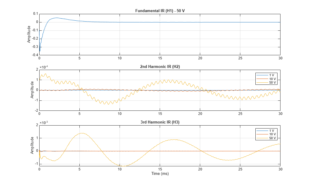
The technique exploits the synchronization property of the sweep: each harmonic of the swept sine is a time-shifted copy of the fundamental. After passing through a nonlinear system, these harmonics appear as distinct, time-separated impulse responses in the output. The function impzest uses this property to cleanly separate the impulse response of each harmonic distortion order from a single measurement.

Model Overview

Open the Simulink model. It consists of a voltage source driving a moving coil speaker in a free-air (unmounted) configuration, with radiation impedance and a far-field pressure sensor.

model = "SweeptoneNonlinearSpeaker";
open_system(model)

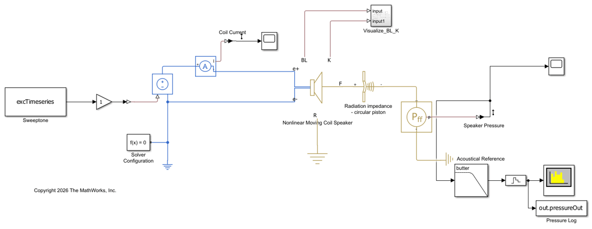
The speaker block has displacement-dependent nonlinearities enabled:

BL(x): Force factor varies with cone displacement (polynomial in x)
K(x): Suspension stiffness varies with cone displacement

These are the dominant nonlinear mechanisms in real loudspeakers. At low drive levels the displacement is small and the system behaves approximately linearly. As the drive level increases, larger cone excursions activate the nonlinear terms, producing measurable harmonic distortion.

Generate the Excitation Signal

Create a synchronized exponential swept sine using sweeptone. The signal sweeps from 20 Hz to 7 kHz over 3 seconds, followed by 2 seconds of silence to capture the impulse response tail. The upper frequency is chosen so that the 2nd and 3rd harmonic responses (up to 14 kHz and 21 kHz) remain below the Nyquist frequency, reducing aliasing and supporting clean harmonic separation.

The excitation signal is created here in the workspace as a timeseries. The Simulink model reads it via a From Workspace block and logs the output pressure via a To Workspace block. Both signals are then used for post-processing with impzest.

fs = 44100;
sweepDuration = 3;
silenceDuration = 2;
sweepRange = [20 7000];
exc = sweeptone(sweepDuration, silenceDuration, fs, ...
    ExcitationLevel=-6, SweepFrequencyRange=sweepRange);

% Create timeseries and sample time for the From Workspace block
Ts = 1/fs;
t = (0:length(exc)-1)'/fs;
excTimeseries = timeseries(exc, t);

totalDuration = length(exc)/fs;

Simulate at Three Nonlinear Drive Levels

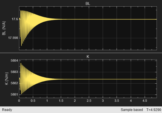
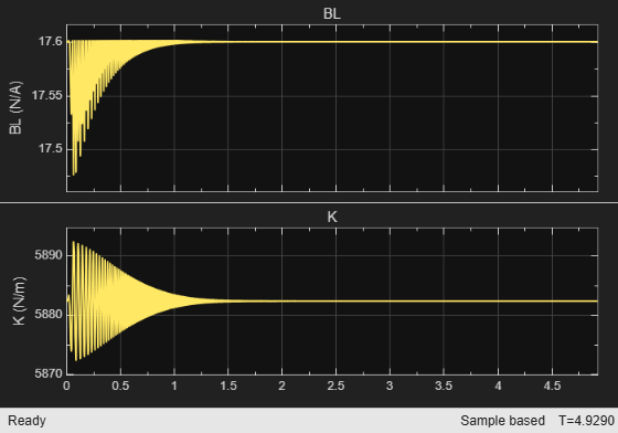
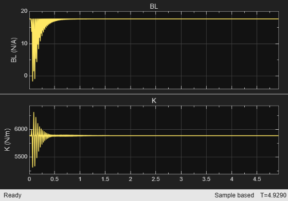
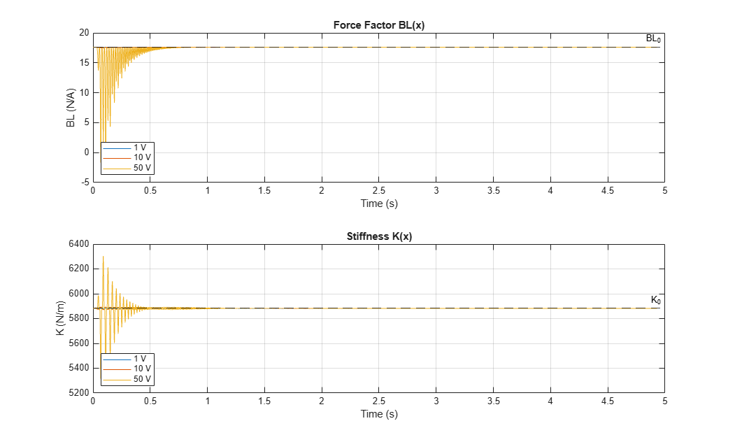
Run the model at increasing drive voltages with BL(x) and K(x) nonlinearities enabled. The BL and K scope opens during simulation, showing how the force factor and stiffness vary with cone displacement in real time. At 1 V the displacement remains in the linear region. At 10 V the nonlinearities are mild. At 50 V the speaker is driven deep into its nonlinear region.

set_param(model, StopTime=num2str(totalDuration), ...
    MaxStep=num2str(1/fs));

driveLevels = [1, 10, 50]; % Volts
simResults = cell(1, 3);

Simulate at 1 V (Linear Region)

set_param(model+"/Gain", Gain="1");
simResults{1} = sim(model);

Simulate at 10 V (Mild Nonlinearity)

set_param(model+"/Gain", Gain="10");
simResults{2} = sim(model);

Simulate at 50 V (Deep Nonlinear Region)

set_param(model+"/Gain", Gain="50");
simResults{3} = sim(model);

Run a Linear Baseline

Disable all nonlinearities and simulate at a moderate drive level (10 V) to establish a truly linear reference. This shows that the harmonics measured above are genuinely caused by the BL(x) and K(x) nonlinearities and not numerical artifacts.

set_param(model+"/Nonlinear Moving Coil Speaker", ...
    BLChoice="false", KChoice="false");
set_param(model+"/Gain", Gain="10");
set_param(model+"/Visualize_BL_K", Commented="on");

simLinear = sim(model);

% Restore nonlinear settings
set_param(model+"/Nonlinear Moving Coil Speaker", ...
    BLChoice="true", KChoice="true");
set_param(model+"/Visualize_BL_K", Commented="off");

Observe BL(x) and K(x) Variation

The model logs the instantaneous force factor and stiffness. At 50 V, the force factor drops by ~40% at peak displacement while the stiffness varies by ~6%. At 1 V, both are essentially constant.

figure
tiledlayout(2,1)

nexttile
for k = 1:3
    plot(simResults{k}.BL_out.Time, simResults{k}.BL_out.Data)
    hold on
end
yline(17.6, "k--", "BL_0")
hold off; grid on
xlabel("Time (s)")
ylabel("BL (N/A)")
title("Force Factor BL(x)")
legend(compose("%d V", driveLevels), Location="southwest")

nexttile
for k = 1:3
    plot(simResults{k}.K_out.Time, simResults{k}.K_out.Data)
    hold on
end
yline(1/0.00017, "k--", "K_0")
hold off; grid on
xlabel("Time (s)")
ylabel("K (N/m)")
title("Stiffness K(x)")
legend(compose("%d V", driveLevels), Location="southwest")

Extract the Pressure Output

The model includes an anti-aliasing filter and zero-order hold that discretize the continuous pressure signal at the audio sample rate, mirroring a real measurement ADC. The To Workspace block logs this discrete signal directly, so no post-processing resampling is needed.

nSamples = min(length(exc), length(simResults{1}.pressureOut.Data));
pressure = zeros(nSamples, 3);

for k = 1:3
    pressure(:,k) = simResults{k}.pressureOut.Data(1:nSamples);
end

% Linear baseline
pressureLinear = simLinear.pressureOut.Data(1:nSamples);

% Trim excitation to match
exc = exc(1:nSamples);

Estimate Impulse Responses and Harmonic Components

Use impzest to estimate the system impulse response and extract individual harmonic distortion impulse responses (H2 and H3). The synchronized sweep property enables clean separation of each harmonic order. "irAll{k} contains the fundamental impulse response, and hAll{k}{n} contains the impulse response of harmonic order n+1.

numHarmonics = 3;

irAll = cell(1,3);
hAll = cell(1,3);

for k = 1:3
    [irAll{k}, hAll{k}] = impzest(exc, pressure(:,k), ...
        NumHarmonics=numHarmonics, ...
        SweepFrequencyRange=sweepRange, SampleRate=fs);
end

% Linear baseline
[irLinear, hLinear] = impzest(exc, pressureLinear, ...
    NumHarmonics=numHarmonics, ...
    SweepFrequencyRange=sweepRange, SampleRate=fs);

Compare Fundamental Frequency Responses

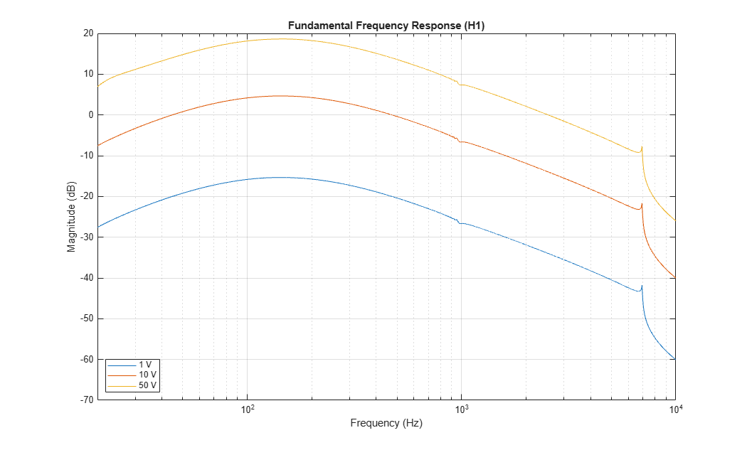
Plot the magnitude response of the fundamental (H1) for all three drive levels. The shape is similar across levels, but at 50 V the response shows subtle gain compression from the BL reduction at large displacements.

nfft = 2^16;
f = (0:nfft/2-1)*fs/nfft;

figure
for k = 1:3
    H1 = 20*log10(abs(fft(irAll{k}, nfft)));
    semilogx(f, H1(1:nfft/2))
    hold on
end
hold off
xlim([20 10000])
grid on
xlabel("Frequency (Hz)")
ylabel("Magnitude (dB)")
title("Fundamental Frequency Response (H1)")
legend(compose("%d V", driveLevels), Location="southwest")

Compare Harmonic Distortion (Relative to Fundamental)

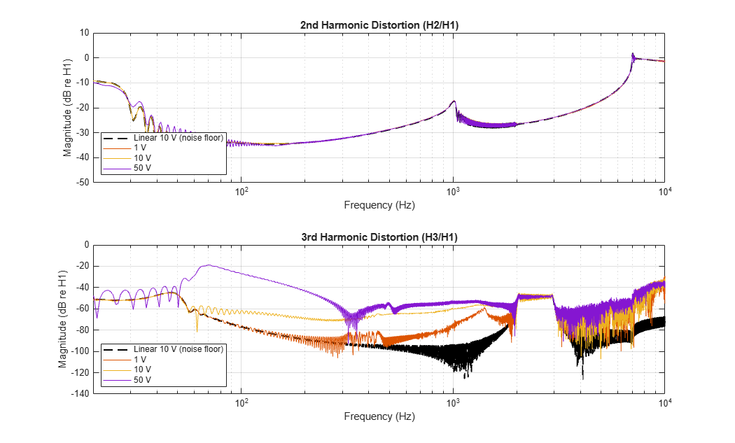
The black dashed line shows the linear baseline at 10 V - this is the numerical noise floor of the simulation. Any harmonic energy above this line is real distortion produced by the BL(x) and K(x) nonlinearities.

Plotting harmonics relative to the fundamental (dB below H1) makes the distortion level directly comparable across drive voltages. H3 grows much faster with level than H2 because it is dominated by the symmetric K(x) terms that only activate at large excursions.

figure
tiledlayout(2,1)

nexttile
% Compute H1 for each level as normalization reference
H1_lin = abs(fft(irLinear, nfft));
H2_lin = abs(fft(hLinear{1}, nfft));
semilogx(f, 20*log10(H2_lin(1:nfft/2) ./ max(H1_lin(1:nfft/2), eps)), ...
    "k--", LineWidth=1.5)
hold on
for k = 1:3
    H1_k = abs(fft(irAll{k}, nfft));
    H2_k = abs(fft(hAll{k}{1}, nfft));
    semilogx(f, 20*log10(H2_k(1:nfft/2) ./ max(H1_k(1:nfft/2), eps)))
end
hold off
xlim([20 10000])
grid on
xlabel("Frequency (Hz)")
ylabel("Magnitude (dB re H1)")
title("2nd Harmonic Distortion (H2/H1)")
legend(["Linear 10 V (noise floor)", compose("%d V", driveLevels)], ...
    Location="southwest")

nexttile
H3_lin = abs(fft(hLinear{2}, nfft));
semilogx(f, 20*log10(H3_lin(1:nfft/2) ./ max(H1_lin(1:nfft/2), eps)), ...
    "k--", LineWidth=1.5)
hold on
for k = 1:3
    H1_k = abs(fft(irAll{k}, nfft));
    H3_k = abs(fft(hAll{k}{2}, nfft));
    semilogx(f, 20*log10(H3_k(1:nfft/2) ./ max(H1_k(1:nfft/2), eps)))
end
hold off
xlim([20 10000])
grid on
xlabel("Frequency (Hz)")
ylabel("Magnitude (dB re H1)")
title("3rd Harmonic Distortion (H3/H1)")
legend(["Linear 10 V (noise floor)", compose("%d V", driveLevels)], ...
    Location="southwest")

Total Harmonic Distortion vs Frequency

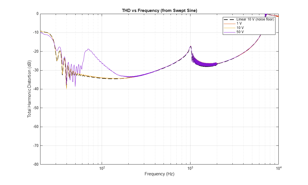
Compute the THD in dB as the ratio of the combined harmonic power to the fundamental power. The swept sine measurement captures THD across the entire frequency range in a single pass - equivalent to running thd at every frequency using a stepped single-tone approach, but far faster.

At 1 V and 10 V the THD falls on the simulation noise floor (matching the linear baseline), confirming that these levels keep the speaker in its linear region. Only at 50 V does the THD rise significantly above the noise floor, reaching approximately -20 dB in the 100-500 Hz range.

figure

% Linear baseline THD
H1_fft_lin = abs(fft(irLinear, nfft));
harmonicPowerLin = zeros(nfft, 1);
for n = 1:numel(hLinear)
    harmonicPowerLin = harmonicPowerLin + abs(fft(hLinear{n}, nfft)).^2;
end
THD_lin_dB = 10*log10(harmonicPowerLin ./ max(H1_fft_lin.^2, eps));
semilogx(f, THD_lin_dB(1:nfft/2), "k--", LineWidth=1.5)
hold on

% Nonlinear cases
for k = 1:3
    H1_fft = abs(fft(irAll{k}, nfft));
    harmonicPower = zeros(nfft, 1);
    for n = 1:numel(hAll{k})
        harmonicPower = harmonicPower + abs(fft(hAll{k}{n}, nfft)).^2;
    end
    THD_dB = 10*log10(harmonicPower ./ max(H1_fft.^2, eps));
    semilogx(f, THD_dB(1:nfft/2))
end
hold off
xlim([20 10000])
ylim([-80 0])
grid on
xlabel("Frequency (Hz)")
ylabel("Total Harmonic Distortion (dB)")
title("THD vs Frequency (from Swept Sine)")
legend(["Linear 10 V (noise floor)", compose("%d V", driveLevels)], ...
    Location="northeast")

Harmonic Impulse Response Separation

The swept sine technique separates each harmonic into its own impulse response. At 1 V the H2 and H3 impulse responses are barely visible. By a gain of 50 V, distinct harmonic impulse responses are visible.

figure
tiledlayout(3,1)
tms = @(x) (0:length(x)-1)/fs*1000;

nexttile
plot(tms(irAll{3}), irAll{3})
xlim([0 30]); grid on
ylabel("Amplitude")
title("Fundamental IR (H1) - 50 V")

nexttile
for k = 1:3
    plot(tms(hAll{k}{1}), hAll{k}{1})
    hold on
end
hold off
xlim([0 30]); grid on
ylabel("Amplitude")
title("2nd Harmonic IR (H2)")
legend(compose("%d V", driveLevels))

nexttile
for k = 1:3
    plot(tms(hAll{k}{2}), hAll{k}{2})
    hold on
end
hold off
xlim([0 30]); grid on
ylabel("Amplitude")
xlabel("Time (ms)")
title("3rd Harmonic IR (H3)")
legend(compose("%d V", driveLevels))

Summary

This example demonstrated how to:

Use sweeptone to generate a synchronized exponential swept sine suitable for nonlinear system identification.
Simulate a Simscape Acoustics loudspeaker model with displacement-dependent BL(x) and K(x) nonlinearities at multiple drive levels.
Observe the time-varying BL(x) and K(x) directly from the model, showing how excursion drives the speaker into its nonlinear region.
Use impzest to extract the fundamental impulse response and individual harmonic distortion impulse responses (H2, H3) from a single measurement.
Compute THD vs frequency from the swept sine measurement in a single pass.
Visualize how harmonic distortion increases with drive level, confirming the nonlinear behavior of the speaker model.

The swept sine method is widely used in loudspeaker characterization because a single measurement captures the complete nonlinear fingerprint of the device under test.

bdclose(model)