Decode J1939 Data from Vector ASC Files
This example shows you how to import and decode J1939 data from Vector ASC files in MATLAB® for analysis. The ASC log and CAN database files used in this example are similar to the files used in the Decode J1939 Data from BLF Files example.
J1939 is a protocol built on top of the CAN protocol. A parameter group (PG) is a set of parameters belonging to the same topic and sharing the same transmission rate e.g. EngCoolantTemp, EngFuelTemp, EngTurboOilTemp, etc. of the ET1_EMS PG (see the ET1_EMS PG in signalTimetables below). Each parameter group is addressed via a unique number called the parameter group number (PGN). J1939 PGs are transmitted as CAN frames.
The ASC file contains data for ChannelID values of 1 and 2, but the J1939 powertrain data of interest was logged from the CAN2 network, so this example will focus on ChannelID 2.
Read J1939 CAN Data Frames from the ASC File
Read all data from channel 2 into a timetable using the canMessageImport function. Each row of the timetable represents one raw CAN frame from the bus.
canData = canMessageImport("LoggingASC_J1939.asc", "Vector", ChannelID=2, OutputFormat="timetable")
canData=26054×8 timetable
       Time           ID        Extended       Name                      Data                    Length      Signals       Error    Remote
    ___________    _________    ________    __________    ___________________________________    ______    ____________    _____    ______

    0.12205 sec    418316262     true       {0×0 char}    {[      105 52 169 232 0 131 0 16]}      8       {0×0 struct}    false    false
    0.39045 sec    418383078     true       {0×0 char}    {[  255 255 255 208 7 255 255 255]}      8       {0×0 struct}    false    false
    0.41035 sec    418383078     true       {0×0 char}    {[  255 255 255 208 7 255 255 255]}      8       {0×0 struct}    false    false
    0.4203 sec     418382822     true       {0×0 char}    {[  255 0 255 255 255 255 255 255]}      8       {0×0 struct}    false    false
    0.42119 sec    419327206     true       {0×0 char}    {[255 255 255 255 255 255 255 255]}      8       {0×0 struct}    false    false
    0.43023 sec    418383078     true       {0×0 char}    {[  255 255 255 208 7 255 255 255]}      8       {0×0 struct}    false    false
    0.45003 sec    418383078     true       {0×0 char}    {[  255 255 255 208 7 255 255 255]}      8       {0×0 struct}    false    false
    0.46988 sec    418382822     true       {0×0 char}    {[  255 0 255 255 255 255 255 255]}      8       {0×0 struct}    false    false
    0.47079 sec    418383078     true       {0×0 char}    {[  255 255 255 208 7 255 255 255]}      8       {0×0 struct}    false    false
    0.47084 sec    419327206     true       {0×0 char}    {[255 255 255 255 255 255 255 255]}      8       {0×0 struct}    false    false
    0.47182 sec    419361254     true       {0×0 char}    {[     255 0 0 12 255 255 224 255]}      8       {0×0 struct}    false    false
    0.48968 sec    418383078     true       {0×0 char}    {[  255 255 255 208 7 255 255 255]}      8       {0×0 struct}    false    false
    0.50949 sec    418383078     true       {0×0 char}    {[  255 255 255 208 7 255 255 255]}      8       {0×0 struct}    false    false
    0.51948 sec    418382822     true       {0×0 char}    {[  255 0 255 255 255 255 255 255]}      8       {0×0 struct}    false    false
    0.52037 sec    419327206     true       {0×0 char}    {[255 255 255 255 255 255 255 255]}      8       {0×0 struct}    false    false
    0.52939 sec    418383078     true       {0×0 char}    {[  255 255 255 208 7 255 255 255]}      8       {0×0 struct}    false    false
      ⋮
Decode J1939 Parameter Groups Using the DBC File
Open the database file using the canDatabase function.
canDB = canDatabase("Powertrain_J1939_ASC.dbc")canDB =
Database with properties:
Name: 'Powertrain_J1939_ASC'
Path: '/tmp/Bdoc26a_3233028_2210314/tp94d33388/vnt-ex98460381/Powertrain_J1939_ASC.dbc'
UTF8_File: '/tmp/Bdoc26a_3233028_2210314/tpa369c5d0_9aa6_4ac9_8b0e_361d636f8c76'
Nodes: {12×1 cell}
NodeInfo: [12×1 struct]
Messages: {93×1 cell}
MessageInfo: [93×1 struct]
Attributes: {3×1 cell}
AttributeInfo: [3×1 struct]
UserData: []
The j1939ParameterGroupTimetable function uses the database to decode the raw CAN Data into PGs, PGNs and signals. The timetable of binary logging format data is converted into a Vehicle Network Toolbox™ J1939 parameter group timetable.
j1939PGTimetable = j1939ParameterGroupTimetable(canData, canDB)
j1939PGTimetable=26054×8 timetable
       Time          Name       PGN     Priority        PDUFormatType        SourceAddress    DestinationAddress                   Data                      Signals
    ___________    ________    _____    ________    _____________________    _____________    __________________    ___________________________________    ____________

    0.12205 sec    ACL         60928       6        Peer-to-Peer (Type 1)         230                255            {[      105 52 169 232 0 131 0 16]}    {1×1 struct}
    0.39045 sec    EEC1_EMS    61444       6        Broadcast (Type 2)            230                255            {[  255 255 255 208 7 255 255 255]}    {1×1 struct}
    0.41035 sec    EEC1_EMS    61444       6        Broadcast (Type 2)            230                255            {[  255 255 255 208 7 255 255 255]}    {1×1 struct}
    0.4203 sec     EEC2_EMS    61443       6        Broadcast (Type 2)            230                255            {[  255 0 255 255 255 255 255 255]}    {1×1 struct}
    0.42119 sec    TCO1_TCO    65132       6        Broadcast (Type 2)            230                255            {[255 255 255 255 255 255 255 255]}    {1×1 struct}
    0.43023 sec    EEC1_EMS    61444       6        Broadcast (Type 2)            230                255            {[  255 255 255 208 7 255 255 255]}    {1×1 struct}
    0.45003 sec    EEC1_EMS    61444       6        Broadcast (Type 2)            230                255            {[  255 255 255 208 7 255 255 255]}    {1×1 struct}
    0.46988 sec    EEC2_EMS    61443       6        Broadcast (Type 2)            230                255            {[  255 0 255 255 255 255 255 255]}    {1×1 struct}
    0.47079 sec    EEC1_EMS    61444       6        Broadcast (Type 2)            230                255            {[  255 255 255 208 7 255 255 255]}    {1×1 struct}
    0.47084 sec    TCO1_TCO    65132       6        Broadcast (Type 2)            230                255            {[255 255 255 255 255 255 255 255]}    {1×1 struct}
    0.47182 sec    CCVS_EMS    65265       6        Broadcast (Type 2)            230                255            {[     255 0 0 12 255 255 224 255]}    {1×1 struct}
    0.48968 sec    EEC1_EMS    61444       6        Broadcast (Type 2)            230                255            {[  255 255 255 208 7 255 255 255]}    {1×1 struct}
    0.50949 sec    EEC1_EMS    61444       6        Broadcast (Type 2)            230                255            {[  255 255 255 208 7 255 255 255]}    {1×1 struct}
    0.51948 sec    EEC2_EMS    61443       6        Broadcast (Type 2)            230                255            {[  255 0 255 255 255 255 255 255]}    {1×1 struct}
    0.52037 sec    TCO1_TCO    65132       6        Broadcast (Type 2)            230                255            {[255 255 255 255 255 255 255 255]}    {1×1 struct}
    0.52939 sec    EEC1_EMS    61444       6        Broadcast (Type 2)            230                255            {[  255 255 255 208 7 255 255 255]}    {1×1 struct}
      ⋮
View the signal data stored in the third PG of the timetable, which is one instance of the "EEC1_EMS" PG.
signalData = j1939PGTimetable.Signals{3}signalData = struct with fields:
EngDemandPercentTorque: 130
EngStarterMode: 15
SrcAddrssOfCtrllngDvcForEngCtrl: 255
EngSpeed: 250
ActualEngPercentTorque: 130
DriversDemandEngPercentTorque: 130
EngTorqueMode: 15
Repackage and Visualize Signal Values of Interest
Use the j1939SignalTimetable function to repackage signal data from each unique PGN on the bus into a signal timetable. This example creates two individual signal timetables for the two PGs of interest, "EEC1_EMS" and "TCO1_TCO", from the J1939 PG timetable.
signalTimetable1 = j1939SignalTimetable(j1939PGTimetable, ParameterGroups="EEC1_EMS")signalTimetable1=12043×7 timetable
Time EngDemandPercentTorque EngStarterMode SrcAddrssOfCtrllngDvcForEngCtrl EngSpeed ActualEngPercentTorque DriversDemandEngPercentTorque EngTorqueMode
___________ ______________________ ______________ _______________________________ ________ ______________________ _____________________________ _____________
0.39045 sec 130 15 255 250 130 130 15
0.41035 sec 130 15 255 250 130 130 15
0.43023 sec 130 15 255 250 130 130 15
0.45003 sec 130 15 255 250 130 130 15
0.47079 sec 130 15 255 250 130 130 15
0.48968 sec 130 15 255 250 130 130 15
0.50949 sec 130 15 255 250 130 130 15
0.52939 sec 130 15 255 250 130 130 15
0.54922 sec 130 15 255 250 130 130 15
0.56999 sec 130 15 255 250 130 130 15
0.5888 sec 130 15 255 250 130 130 15
0.60868 sec 130 15 255 250 130 130 15
0.6285 sec 130 15 255 250 130 130 15
0.64833 sec 130 15 255 250 130 130 15
0.66918 sec 130 15 255 250 130 130 15
0.68804 sec 130 15 255 250 130 130 15
⋮
signalTimetable2 = j1939SignalTimetable(j1939PGTimetable, ParameterGroups="TCO1_TCO")signalTimetable2=4817×14 timetable
Time TachographVehicleSpeed TachographOutputShaftSpeed DirectionIndicator TachographPerformance HandlingInformation SystemEvent DriverCardDriver2 Driver2TimeRelatedStates Overspeed DriverCardDriver1 Driver1TimeRelatedStates DriveRecognize Driver2WorkingState Driver1WorkingState
___________ ______________________ __________________________ __________________ _____________________ ___________________ ___________ _________________ ________________________ _________ _________________ ________________________ ______________ ___________________ ___________________
0.42119 sec 256 8191.9 3 3 3 3 3 15 3 3 15 3 7 7
0.47084 sec 256 8191.9 3 3 3 3 3 15 3 3 15 3 7 7
0.52037 sec 256 8191.9 3 3 3 3 3 15 3 3 15 3 7 7
0.57008 sec 256 8191.9 3 3 3 3 3 15 3 3 15 3 7 7
0.61952 sec 256 8191.9 3 3 3 3 3 15 3 3 15 3 7 7
0.66922 sec 256 8191.9 3 3 3 3 3 15 3 3 15 3 7 7
0.71886 sec 256 8191.9 3 3 3 3 3 15 3 3 15 3 7 7
0.76874 sec 256 8191.9 3 3 3 3 3 15 3 3 15 3 7 7
0.81827 sec 256 8191.9 3 3 3 3 3 15 3 3 15 3 7 7
0.86808 sec 256 8191.9 3 3 3 3 3 15 3 3 15 3 7 7
0.91762 sec 256 8191.9 3 3 3 3 3 15 3 3 15 3 7 7
0.96737 sec 256 8191.9 3 3 3 3 3 15 3 3 15 3 7 7
1.0169 sec 256 8191.9 3 3 3 3 3 15 3 3 15 3 7 7
1.0667 sec 256 8191.9 3 3 3 3 3 15 3 3 15 3 7 7
1.116 sec 256 8191.9 3 3 3 3 3 15 3 3 15 3 7 7
1.1656 sec 256 8191.9 3 3 3 3 3 15 3 3 15 3 7 7
⋮
You can alternatively choose to convert the whole J1939 PG timetable into a struct containing multiple J1939 signal timetables for each individual PG, and index into it to get data for a particular PG.
signalTimetables = j1939SignalTimetable(j1939PGTimetable)
signalTimetables = struct with fields:
          ACL: [1×14 timetable]
     CCVS_EMS: [2408×19 timetable]
           DD: [240×5 timetable]
     EEC1_EMS: [12043×7 timetable]
     EEC2_EMS: [4817×10 timetable]
      ET1_EMS: [240×6 timetable]
    HOURS_EMS: [240×2 timetable]
      LFC_EMS: [480×2 timetable]
         SERV: [240×6 timetable]
     TCO1_TCO: [4817×14 timetable]
     VDHR_EMS: [240×2 timetable]
       VI_EMS: [24×1 timetable]
       VW_SSC: [240×4 timetable]
signalTimetables.EEC1_EMS
ans=12043×7 timetable
       Time        EngDemandPercentTorque    EngStarterMode    SrcAddrssOfCtrllngDvcForEngCtrl    EngSpeed    ActualEngPercentTorque    DriversDemandEngPercentTorque    EngTorqueMode
    ___________    ______________________    ______________    _______________________________    ________    ______________________    _____________________________    _____________

    0.39045 sec             130                    15                        255                    250                130                           130                      15
    0.41035 sec             130                    15                        255                    250                130                           130                      15
    0.43023 sec             130                    15                        255                    250                130                           130                      15
    0.45003 sec             130                    15                        255                    250                130                           130                      15
    0.47079 sec             130                    15                        255                    250                130                           130                      15
    0.48968 sec             130                    15                        255                    250                130                           130                      15
    0.50949 sec             130                    15                        255                    250                130                           130                      15
    0.52939 sec             130                    15                        255                    250                130                           130                      15
    0.54922 sec             130                    15                        255                    250                130                           130                      15
    0.56999 sec             130                    15                        255                    250                130                           130                      15
    0.5888 sec              130                    15                        255                    250                130                           130                      15
    0.60868 sec             130                    15                        255                    250                130                           130                      15
    0.6285 sec              130                    15                        255                    250                130                           130                      15
    0.64833 sec             130                    15                        255                    250                130                           130                      15
    0.66918 sec             130                    15                        255                    250                130                           130                      15
    0.68804 sec             130                    15                        255                    250                130                           130                      15
      ⋮
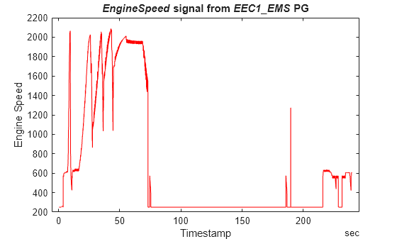
To visualize a signal of interest, variables from the signal timetables can be plotted over time for further analysis. For this example, look at the "EngineSpeed" signal from the "EEC1_EMS" PG.
plot(signalTimetable1.Time, signalTimetable1.EngSpeed, "r")
title("{\itEngineSpeed} signal from {\itEEC1\_EMS} PG", FontWeight="bold")
xlabel("Timestamp")
ylabel("Engine Speed")
Alternative Method to Read and Decode
The function j1939ParameterGroupImport can be used instead of using canMessageImport and j1939ParameterGroupTimetable to read and decode J1939 data from ASC files in one step.
j1939PGTimetable = j1939ParameterGroupImport("LoggingASC_J1939.asc", "Vector", canDB, ChannelID=2)
j1939PGTimetable=26054×8 timetable
       Time          Name       PGN     Priority        PDUFormatType        SourceAddress    DestinationAddress                   Data                      Signals
    ___________    ________    _____    ________    _____________________    _____________    __________________    ___________________________________    ____________

    0.12205 sec    ACL         60928       6        Peer-to-Peer (Type 1)         230                255            {[      105 52 169 232 0 131 0 16]}    {1×1 struct}
    0.39045 sec    EEC1_EMS    61444       6        Broadcast (Type 2)            230                255            {[  255 255 255 208 7 255 255 255]}    {1×1 struct}
    0.41035 sec    EEC1_EMS    61444       6        Broadcast (Type 2)            230                255            {[  255 255 255 208 7 255 255 255]}    {1×1 struct}
    0.4203 sec     EEC2_EMS    61443       6        Broadcast (Type 2)            230                255            {[  255 0 255 255 255 255 255 255]}    {1×1 struct}
    0.42119 sec    TCO1_TCO    65132       6        Broadcast (Type 2)            230                255            {[255 255 255 255 255 255 255 255]}    {1×1 struct}
    0.43023 sec    EEC1_EMS    61444       6        Broadcast (Type 2)            230                255            {[  255 255 255 208 7 255 255 255]}    {1×1 struct}
    0.45003 sec    EEC1_EMS    61444       6        Broadcast (Type 2)            230                255            {[  255 255 255 208 7 255 255 255]}    {1×1 struct}
    0.46988 sec    EEC2_EMS    61443       6        Broadcast (Type 2)            230                255            {[  255 0 255 255 255 255 255 255]}    {1×1 struct}
    0.47079 sec    EEC1_EMS    61444       6        Broadcast (Type 2)            230                255            {[  255 255 255 208 7 255 255 255]}    {1×1 struct}
    0.47084 sec    TCO1_TCO    65132       6        Broadcast (Type 2)            230                255            {[255 255 255 255 255 255 255 255]}    {1×1 struct}
    0.47182 sec    CCVS_EMS    65265       6        Broadcast (Type 2)            230                255            {[     255 0 0 12 255 255 224 255]}    {1×1 struct}
    0.48968 sec    EEC1_EMS    61444       6        Broadcast (Type 2)            230                255            {[  255 255 255 208 7 255 255 255]}    {1×1 struct}
    0.50949 sec    EEC1_EMS    61444       6        Broadcast (Type 2)            230                255            {[  255 255 255 208 7 255 255 255]}    {1×1 struct}
    0.51948 sec    EEC2_EMS    61443       6        Broadcast (Type 2)            230                255            {[  255 0 255 255 255 255 255 255]}    {1×1 struct}
    0.52037 sec    TCO1_TCO    65132       6        Broadcast (Type 2)            230                255            {[255 255 255 255 255 255 255 255]}    {1×1 struct}
    0.52939 sec    EEC1_EMS    61444       6        Broadcast (Type 2)            230                255            {[  255 255 255 208 7 255 255 255]}    {1×1 struct}
      ⋮
The signals in this timetable can be repackaged and visualized the same as above.