部分木の標本外応答の予測
この例では、回帰木の標本外応答を予測して結果をプロットする方法を示します。
carsmall データ セットを読み込みます。Weight が応答 MPG の予測子であると考えます。
load carsmall
idxNaN = isnan(MPG + Weight);
X = Weight(~idxNaN);
Y = MPG(~idxNaN);
n = numel(X);
データを学習セット (50%) と検証セット (50%) に分割します。
rng(1) % For reproducibility
idxTrn = false(n,1);
idxTrn(randsample(n,round(0.5*n))) = true; % Training set logical indices
idxVal = idxTrn == false;                  % Validation set logical indices
学習観測値を使用して回帰木を成長させます。
Mdl = fitrtree(X(idxTrn),Y(idxTrn));
view(Mdl,'Mode','graph')
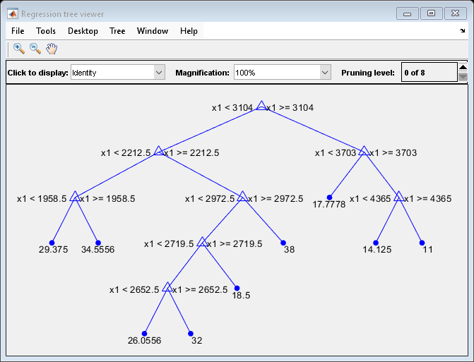
いくつかの部分木ごとに検証観測値の近似値を計算します。
m = max(Mdl.PruneList);
pruneLevels = 0:2:m; % Pruning levels to consider
z = numel(pruneLevels);
Yfit = predict(Mdl,X(idxVal),'SubTrees',pruneLevels);
Yfit は、近似値が含まれている n 行 z 列の行列です。各行は観測値に、各列は部分木に対応しています。
Yfit と Y を X に対してプロットします。
figure;
sortDat = sortrows([X(idxVal) Y(idxVal) Yfit],1); % Sort all data with respect to X
plot(sortDat(:,1),sortDat(:,2),'*');
hold on;
plot(repmat(sortDat(:,1),1,size(Yfit,2)),sortDat(:,3:end));
lev = cellstr(num2str((pruneLevels)','Level %d MPG'));
legend(['Observed MPG'; lev])
title 'Out-of-Sample Predictions'
xlabel 'Weight (lbs)';
ylabel 'MPG';
h = findobj(gcf);
axis tight;
set(h(4:end),'LineWidth',3) % Widen all lines
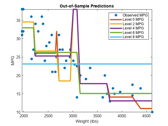
下位の枝刈りレベルでは、Yfit の値が上位レベルよりデータに近づく傾向があります。上位の枝刈りレベルでは、X の間隔が大きくなるのでフラットになる傾向があります。