線形混合効果モデルのワークフロー
R2026bこの例では、LME (線形混合効果モデル) の当てはめと解析の方法を説明します。
標本データを読み込みます。
load fluTable
flu
flu = 52×11 table
Date NE MidAtl ENCentral WNCentral SAtl ESCentral WSCentral Mtn Pac WtdILI
______________ _____ ______ _________ _________ _____ _________ _________ _____ _____ ______
{'10/9/2005' } 0.97 1.025 1.232 1.286 1.082 1.457 1.1 0.981 0.971 1.182
{'10/16/2005'} 1.136 1.06 1.228 1.286 1.146 1.644 1.123 0.976 0.917 1.22
{'10/23/2005'} 1.135 1.172 1.278 1.536 1.274 1.556 1.236 1.102 0.895 1.31
{'10/30/2005'} 1.52 1.489 1.576 1.794 1.59 2.252 1.612 1.321 1.082 1.343
{'11/6/2005' } 1.365 1.394 1.53 1.825 1.62 2.059 1.471 1.453 1.118 1.586
{'11/13/2005'} 1.39 1.477 1.506 1.9 1.683 1.813 1.464 1.388 1.204 1.47
{'11/20/2005'} 1.212 1.231 1.295 1.495 1.347 1.794 1.303 1.371 1.137 1.611
{'11/27/2005'} 1.477 1.546 1.557 1.855 1.678 2.159 1.739 1.628 1.443 1.827
{'12/4/2005' } 1.285 1.43 1.482 1.635 1.577 1.903 1.53 1.701 1.516 1.776
{'12/11/2005'} 1.354 1.45 1.46 1.794 1.583 1.894 1.831 2.364 2.094 1.941
{'12/18/2005'} 1.502 1.622 1.638 1.988 1.947 2.22 2.577 3.89 2.66 2.34
{'12/25/2005'} 1.86 1.915 1.955 2.38 2.343 3.027 3.219 4.862 2.595 3.086
{'1/1/2006' } 2.114 2.174 2.065 2.557 2.275 2.498 2.644 3.352 2.181 3.26
{'1/8/2006' } 1.815 1.932 1.822 2.046 1.969 1.805 2.189 2.132 1.717 2.613
{'1/15/2006' } 1.541 1.695 1.581 2.008 1.718 1.662 2.156 1.694 1.351 2.247
{'1/22/2006' } 1.632 1.758 1.711 2.217 1.866 2.194 2.268 1.826 1.384 2.352
⋮
データセット配列 flu には、変数 Date と、インフルエンザ推定罹患率 (Google® 検索から推定される 9 地域の値と CDC による全国の推定値) が格納されている 10 個の変数が含まれています。
データを再編成してプロットする
線形混合効果モデルを当てはめるには、データが適切な形式の table になっていなければなりません。インフルエンザ羅患率を応答として使用することにより線形混合効果モデルを当てはめるには、地域に対応する 9 個の列を 1 つの配列にまとめます。新しいデータセット配列 flu2 には、応答変数 FluRate、各推定の元になっている地域を示すノミナル変数 Region、全国の推定値 WtdILI およびグループ化変数 Date が含まれなければなりません。
flu2 = stack(flu,2:10,NewDataVariableName="FluRate",...
    IndexVariableName="Region");
flu2.Date = nominal(flu2.Date);
flu2.Region = nominal(flu2.Region);
インフルエンザ罹患率を全国の推定値に対してプロットします。
plot(flu2.WtdILI,flu2.FluRate,"ro")
xlabel("WtdILI")
ylabel("Flu Rate")
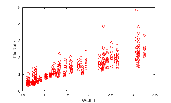
プロットから、各地域のインフルエンザ罹患率は全国の推定値と直接的な関係があることがわかります。
LME モデルを当てはめて結果を解釈する
全国の推定値を予測子変数として使用し、Date で変化するランダム切片で線形混合効果モデルを当てはめます。
rng(0,"twister") % For reproducibility
lme = fitlme(flu2,"FluRate ~ 1 + WtdILI + (1|Date)")
lme =
Linear mixed-effects model fit by ML

Model information:
    Number of observations             468
    Fixed effects coefficients           2
    Random effects coefficients         52
    Covariance parameters                2

Formula:
    FluRate ~ 1 + WtdILI + (1 | Date)

Model fit statistics:
    AIC       BIC       LogLikelihood    Deviance
    286.24    302.83    -139.12          278.24

Fixed effects coefficients (95% CIs):
    Name                   Estimate    SE          tStat     DF     pValue        Lower       Upper
    {'(Intercept)'}        0.16385     0.057525    2.8484    466     0.0045885    0.050813    0.27689
    {'WtdILI'     }         0.7236     0.032219    22.459    466    3.0502e-76     0.66028    0.78691

Random effects covariance parameters (95% CIs):
Group: Date (52 Levels)
    Name1                  Name2                  Type           Estimate    Lower      Upper
    {'(Intercept)'}        {'(Intercept)'}        {'std'}        0.17146     0.13227    0.22226

Group: Error
    Name               Estimate    Lower      Upper
    {'Res Std'}        0.30201     0.28217    0.32324
0.0045885 および 3.0502e-76 という小さい p 値は、切片と全国の推定値の両方が有意であることを示しています。また、変量効果項 の標準偏差の信頼限界 (0.13227, 0.22226) には、変量効果項が有意であることを示す 0 が含まれていません。
生の残差と近似値の対比をプロットします。
figure();
plotResiduals(lme,"fitted")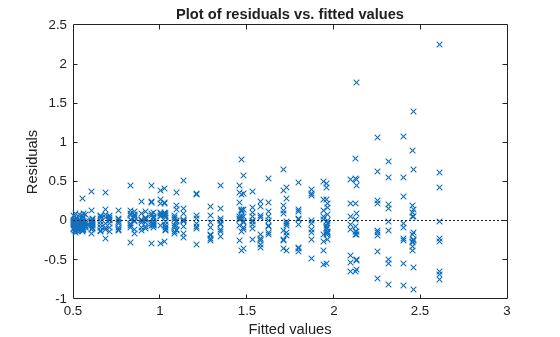
近似応答値の増加にともない残差の分散も増加します。この現象は不均一分散と呼ばれています。
外れ値のように右上に表示されている 2 件の観測値を検出します。
find(residuals(lme) > 1.5)
ans = 2×1

    98
   107
これらの観測値を削除して、モデルを再度当てはめます。
lme = fitlme(flu2,"FluRate ~ 1 + WtdILI + (1|Date)",Exclude=[98,107]);モデルを改良する
Date でグループ化された全国の推定値に独立したランダム項を含めると、モデルが改善されるか判定します。
altlme = fitlme(flu2,"FluRate ~ 1 + WtdILI + (1|Date) + (WtdILI-1|Date)",...
    Exclude=[98,107])
altlme =
Linear mixed-effects model fit by ML

Model information:
    Number of observations             466
    Fixed effects coefficients           2
    Random effects coefficients        104
    Covariance parameters                3

Formula:
    FluRate ~ 1 + WtdILI + (1 | Date) + (WtdILI | Date)

Model fit statistics:
    AIC       BIC       LogLikelihood    Deviance
    179.39    200.11    -84.694          169.39

Fixed effects coefficients (95% CIs):
    Name                   Estimate    SE          tStat     DF     pValue       Lower      Upper
    {'(Intercept)'}        0.17837     0.054585    3.2676    464     0.001165     0.0711    0.28563
    {'WtdILI'     }        0.70836     0.030594    23.153    464    2.123e-79    0.64824    0.76849

Random effects covariance parameters (95% CIs):
Group: Date (52 Levels)
    Name1                  Name2                  Type           Estimate    Lower      Upper
    {'(Intercept)'}        {'(Intercept)'}        {'std'}        0.16631     0.12977    0.21313

Group: Date (52 Levels)
    Name1             Name2             Type           Estimate     Lower    Upper
    {'WtdILI'}        {'WtdILI'}        {'std'}        4.676e-08    NaN      NaN

Group: Error
    Name               Estimate    Lower      Upper
    {'Res Std'}        0.26691     0.24934    0.28572
WtdILI 項の標準偏差の推定値はほぼ 0 なので、信頼区間を計算できません。これは、モデルのパラメーターが多すぎ、(WtdILI-1|Date) 項が有意でないことを示しています。次のように compare メソッドを使用すると、これを正式に検定できます。compare(lme,altlme,CheckNesting=true)。
Region でグループ化された切片の変量効果項を初期モデル lme に追加します。
lme2 = fitlme(flu2,"FluRate ~ 1 + WtdILI + (1|Date) + (1|Region)",...
    Exclude=[98,107]);
lme モデルと lme2 モデルを比較します。
compare(lme,lme2,CheckNesting=true)
ans =
    Theoretical Likelihood Ratio Test

    Model    DF    AIC       BIC       LogLik     LRStat    deltaDF    pValue
    lme      4     177.39    193.97    -84.694
    lme2     5     62.265    82.986    -26.133    117.12    1          0
切片と全国平均に、相関する可能性のある変量効果項を追加すると、モデル lme2 が改善されるか確認します。
lme3 = fitlme(flu2,"FluRate ~ 1 + WtdILI + (1|Date) + (1 + WtdILI|Region)",...
    Exclude=[98,107])
lme3 =
Linear mixed-effects model fit by ML

Model information:
    Number of observations             466
    Fixed effects coefficients           2
    Random effects coefficients         70
    Covariance parameters                5

Formula:
    FluRate ~ 1 + WtdILI + (1 | Date) + (1 + WtdILI | Region)

Model fit statistics:
    AIC       BIC       LogLikelihood    Deviance
    13.338    42.348    0.33076          -0.66153

Fixed effects coefficients (95% CIs):
    Name                   Estimate    SE          tStat     DF     pValue        Lower       Upper
    {'(Intercept)'}         0.1795     0.054953    3.2665    464     0.0011697    0.071514    0.28749
    {'WtdILI'     }        0.70719      0.04252    16.632    464    4.6451e-49     0.62363    0.79074

Random effects covariance parameters (95% CIs):
Group: Date (52 Levels)
    Name1                  Name2                  Type           Estimate    Lower      Upper
    {'(Intercept)'}        {'(Intercept)'}        {'std'}        0.17634     0.14093    0.22064

Group: Region (9 Levels)
    Name1                  Name2                  Type            Estimate     Lower         Upper
    {'(Intercept)'}        {'(Intercept)'}        {'std' }        0.0077037    3.2284e-16    1.8383e+11
    {'WtdILI'     }        {'(Intercept)'}        {'corr'}        -0.059604      -0.99996       0.99995
    {'WtdILI'     }        {'WtdILI'     }        {'std' }         0.088069      0.051694       0.15004

Group: Error
    Name               Estimate    Lower      Upper
    {'Res Std'}        0.20976     0.19568    0.22486
Region でグループ化された切片に関する変量効果項の標準偏差の推定値は 0.0077037 で、信頼区間が非常に大きく、0 が含まれています。これは、Region でグループ化された切片の変量効果が有意でないことを示しています。切片と WtdILI の間で変量効果の相関は –0.059604 です。この相関の信頼区間も非常に大きく、0 が含まれています。これは、相関が有意でないことを示しています。
(1 + WtdILI | Region) 変量効果項から切片を削除して、モデルを再度当てはめます。
lme3 = fitlme(flu2,"FluRate ~ 1 + WtdILI + (1|Date) + (WtdILI - 1|Region)",...
    Exclude=[98,107])
lme3 =
Linear mixed-effects model fit by ML

Model information:
    Number of observations             466
    Fixed effects coefficients           2
    Random effects coefficients         61
    Covariance parameters                3

Formula:
    FluRate ~ 1 + WtdILI + (1 | Date) + (WtdILI | Region)

Model fit statistics:
    AIC       BIC      LogLikelihood    Deviance
    9.3395    30.06    0.33023          -0.66046

Fixed effects coefficients (95% CIs):
    Name                   Estimate    SE          tStat     DF     pValue        Lower       Upper
    {'(Intercept)'}         0.1795     0.054892    3.2702    464     0.0011549    0.071637    0.28737
    {'WtdILI'     }        0.70718     0.042486    16.645    464    4.0496e-49     0.62369    0.79067

Random effects covariance parameters (95% CIs):
Group: Date (52 Levels)
    Name1                  Name2                  Type           Estimate    Lower      Upper
    {'(Intercept)'}        {'(Intercept)'}        {'std'}        0.17633     0.14092    0.22062

Group: Region (9 Levels)
    Name1             Name2             Type           Estimate    Lower       Upper
    {'WtdILI'}        {'WtdILI'}        {'std'}        0.087925    0.054474    0.14192

Group: Error
    Name               Estimate    Lower      Upper
    {'Res Std'}        0.20979     0.19585    0.22473
新しいモデル lme3 の項はすべて有意です。
lme2 と lme3 を比較します。
compare(lme2,lme3,CheckNesting=true,NSim=100)
ans =
    Simulated Likelihood Ratio Test: Nsim = 100, Alpha = 0.05

    Model    DF    AIC       BIC       LogLik     LRStat    pValue      Lower         Upper
    lme2     5     62.265    82.986    -26.133
    lme3     5     9.3395     30.06    0.33023    52.926    0.009901    0.00025064    0.053932
0.009901 という $p$ 値は、lme3 が lme2 より適切に当てはめられていることを示しています。
2 次固定効果項をモデル lme3 に追加します。
lme4 = fitlme(flu2,"FluRate ~ 1 + WtdILI^2 + (1|Date) + (WtdILI - 1|Region)",...
    Exclude=[98,107])
lme4 =
Linear mixed-effects model fit by ML

Model information:
    Number of observations             466
    Fixed effects coefficients           3
    Random effects coefficients         61
    Covariance parameters                3

Formula:
    FluRate ~ 1 + WtdILI + WtdILI^2 + (1 | Date) + (WtdILI | Region)

Model fit statistics:
    AIC       BIC       LogLikelihood    Deviance
    6.7234    31.588    2.6383           -5.2766

Fixed effects coefficients (95% CIs):
    Name                   Estimate     SE         tStat       DF     pValue        Lower       Upper
    {'(Intercept)'}        -0.063406    0.12236    -0.51821    463       0.60456    -0.30385      0.17704
    {'WtdILI'     }           1.0594    0.16554      6.3996    463    3.8232e-10     0.73406       1.3847
    {'WtdILI^2'   }        -0.096919     0.0441     -2.1977    463      0.028463    -0.18358    -0.010259

Random effects covariance parameters (95% CIs):
Group: Date (52 Levels)
    Name1                  Name2                  Type           Estimate    Lower      Upper
    {'(Intercept)'}        {'(Intercept)'}        {'std'}        0.16732     0.13326    0.21009

Group: Region (9 Levels)
    Name1             Name2             Type           Estimate    Lower       Upper
    {'WtdILI'}        {'WtdILI'}        {'std'}        0.087865    0.054443    0.1418

Group: Error
    Name               Estimate    Lower      Upper
    {'Res Std'}        0.20979     0.19585    0.22473
0.028463 という $p$ 値は、2 次項 WtdILI^2 の係数が有意であることを示しています。
近似された応答を観測された応答と残差に対してプロットする
F = fitted(lme4);
R = response(lme4);
figure();
plot(R,F,"rx")
xlabel("Response")
ylabel("Fitted")
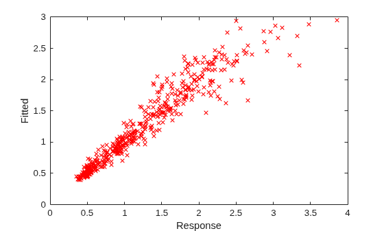
観測された応答と比較すると、近似された応答の値の角度がほぼ 45 度になります。これは近似の精度が高いことを意味します。
残差と近似値の対比をプロットします。
figure();
plotResiduals(lme4,"fitted")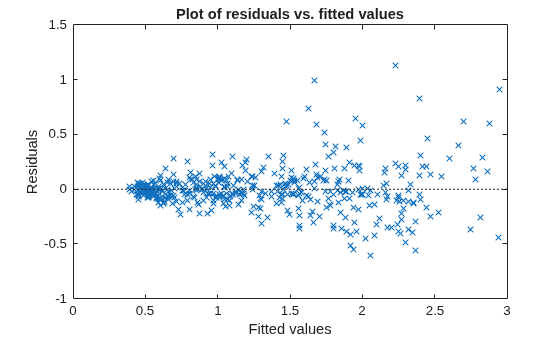
モデルは改善されていますが、まだ不均一分散が認識されます。原因として、データ セットに存在しない (つまり、モデルに存在しない) 別の予測子が考えられます。
地域 ENCentral、日付 11/6/2005 の近似されたインフルエンザ罹患率を特定します。
F(flu2.Region == "ENCentral" & flu2.Date == "11/6/2005")
ans =
1.4860
応答値を無作為に生成する
全国推定値 1.625、地域 MidAtl、日付 4/23/2006 に対する応答値を無作為に生成します。最初に新しい table を定義します。日付と地域は元の table でノミナルであるため、新しい table でも同様に定義しなければなりません。
tblnew = table(1.625,VariableNames="WtdILI");
tblnew.Region = nominal("MidAtl");
tblnew.Date = nominal("4/23/2006");
次に、応答値を生成します。
random(lme4,tblnew)
ans =
1.2679

