混合効果スプライン回帰の近似

この例では、混合効果線形スプライン モデルを当てはめる方法を説明します。

標本データを読み込みます。

load('mespline.mat');

このデータは、シミュレーションされたものです。

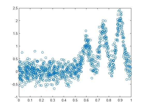
並べ替えられた $$x$$ に対して $$y$$ をプロットします。

[x_sorted,I] = sort(x,'ascend');
plot(x_sorted,y(I),'o')

次の混合効果線形スプライン回帰モデルを当てはめます。

$$y_i={\beta }_1+{\beta }_2{x}_i+\sum _{j=1}^K{b}_j{(x_i-k_j)}_{+}+{ϵ}_i$$

ここで、$$k_j$$ は $$j$$ 番目の節点、$$K$$ は節点の総数です。$$b_j\sim N(0,{\sigma }_b^2)$$ および $$ϵ\sim N(0,{\sigma }^2)$$ であると仮定します。

節点を定義します。

k = linspace(0.05,0.95,100);

計画行列を定義します。

X = [ones(1000,1),x];
Z = zeros(length(x),length(k));
for j = 1:length(k)
      Z(:,j) = max(X(:,2) - k(j),0);
end

変量効果の等方共分散構造によりモデルを当てはめます。

lme = fitlmematrix(X,y,Z,[],'CovariancePattern','Isotropic');

固定効果のみのモデルを当てはめます。

X = [X Z];
lme_fixed = fitlmematrix(X,y,[],[]);

シミュレーションされた尤度比検定を使用して lme_fixed と lme を比較します。

compare(lme,lme_fixed,'NSim',500,'CheckNesting',true)

ans = 
    SIMULATED LIKELIHOOD RATIO TEST: NSIM = 500, ALPHA = 0.05

    Model        DF     AIC       BIC       LogLik     LRStat    pValue     Lower      Upper  
    lme            4    170.62    190.25    -81.309                                           
    lme_fixed    103    113.38    618.88     46.309    255.24    0.68064    0.63784    0.72129

$$p$$ 値は、固定効果のみのモデルが混合効果スプライン回帰モデルよりも適切でない当てはめであることを示しています。

両方のモデルから近似された値を、元の応答データの上部にプロットします。

R = response(lme);
figure();
plot(x_sorted,R(I),'o', 'MarkerFaceColor',[0.8,0.8,0.8],...
    'MarkerEdgeColor',[0.8,0.8,0.8],'MarkerSize',4);
hold on
F = fitted(lme);
F_fixed = fitted(lme_fixed);
plot(x_sorted,F(I),'b');
plot(x_sorted,F_fixed(I),'r');
legend('data','mixed effects','fixed effects','Location','NorthWest')
xlabel('sorted x values');
ylabel('y');
hold off

また、この図からは混合効果モデルの方が固定効果のみのモデルより、データへの当てはめの精度が高くなることもわかります。