Model Cascaded Network
This example shows you how to:
Model a cascaded network,
Analyze the network in the frequency domain
Plot the results.
This example uses a cascaded network that consists of an amplifier and two transmission lines.
Video Walkthrough
For a walkthrough of the example, play the video.
Create RF Components
Create the RF components for the cascaded network. This example shows how to connect two transmission lines and the amplifier in a cascaded network.
FirstCkt = txlineEquationBased;
SecondCkt = amplifier;
ThirdCkt = txlineEquationBased;
Specify Component Data
Specify the transmission line and amplifier properties.
Transmission Line Properties
Set the line length of the first transmission line, FirstCkt, to 1 meters.
FirstCkt.LineLength = 1;
Set the line length of the second transmission line, ThirdCkt, to 0.025 meters and the phase velocity to 2.0e8 m/sec.
ThirdCkt.LineLength = 0.025;
ThirdCkt.PhaseVelocity = 2.0e8;
Amplifier Properties
Import network parameters and noise data from the defaultAmplifier.s2p file into the amplifier, SecondCkt.
SecondCkt.UseNetworkData = true;
SecondCkt.FileName = 'defaultAmplifier.s2p';
Validate RF Components
In this part of the example, you plot the network parameters and power data (output power versus input power) to validate the behavior of the amplifier. Use the smithplot function to plot the original S11 and S22 parameters of the amplifier (SecondCkt) on a Z Smith® Chart.
figure
smithplot(SecondCkt.NetworkData,[1,1;2,2]);
Build and Analyze Cascaded Network
In this part of the example, you create a rfbudget object to represent the cascaded amplifier and analyze the object in the frequency domain. Cascade the three circuit objects to form a new cascaded rfbudget object, CascadedCkt.
CascadedCkt = circuit([FirstCkt SecondCkt ThirdCkt]);
CascadedCkt_S = sparameters(CascadedCkt, SecondCkt.NetworkData.Frequencies);
Analyze Simulation Results
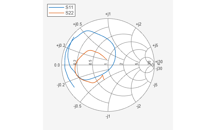
In this part of the example, you analyze the results of the simulation by plotting data for the rfbudget object that represents the cascaded amplifier network. Use the smithplot function to plot the S11 and S22 parameters of the cascaded amplifier network on a Z Smith Chart.
figure
smithplot(CascadedCkt_S,[1,1;2,2]);
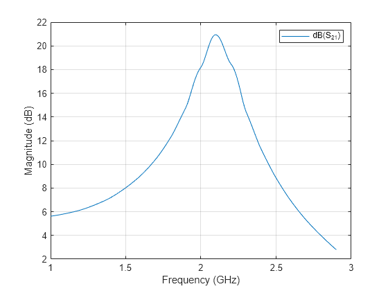
Use the rfplot function to plot the S21 parameter of the cascaded network, which represents the network gain, on an X-Y plane.
rfplot(CascadedCkt_S,2,1)
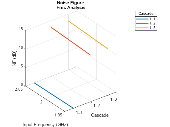
Use the rfplot function to create the noise figure of the cascaded amplifier network.
CascadedBudget = rfbudget([FirstCkt SecondCkt ThirdCkt], 2e9, -30, 100e6);
rfplot(CascadedBudget,'NF')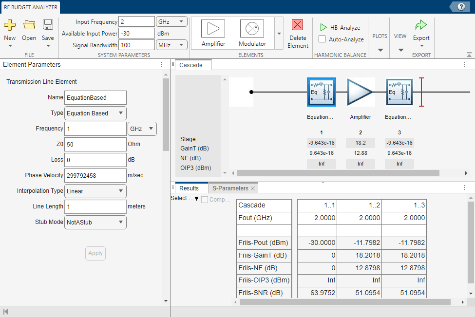
To visualize cascade network and plot S-parameters at each stage, use the RF Budget Analyzer app. Type the rfBudgetAnalyzer(CascadedBudget) command at the command line.
rfBudgetAnalyzer(CascadedBudget)
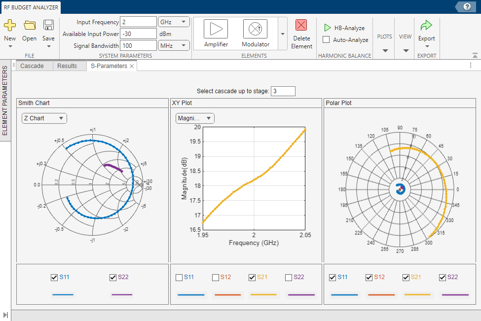
Select S-Parameters Plot button from the Plots section. This allows you to plot Smith® chart, polar plot, magnitude, phase and real, and imaginary parts of S-parameters of the RF System and over stages. Specify 3 in the Select cascade up to stage parameter.
