海上レーダーの海面クラッター モデリング

この例では、海上監視レーダー システムにおける海面クラッターのシミュレーションについて説明します。この例ではまず、海面状態に関連する物理的性質について説明します。次に、海面状態、周波数、偏波、グレージング角の影響を調査しながら、海面反射率について説明します。最後に、この例では、伝播パスと気象の影響を考慮して、海上監視レーダー システムの C/N 比 (CNR) を計算します。

海面状態の概要

海面クラッターを記述するにあたり、まず海面の物理的性質を確立することが重要です。レーダーにおける海面クラッターのモデル化において、3 つの重要なパラメーターがあります。

1. ${\sigma }_h$ は波高の標準偏差。波高とは、波の頂上と隣接する波の谷との間の垂直距離として定義されます。

2. ${\beta }_0$ は波の傾き。

3. $v_w$ は風速。

波の不規則性のため、海の物理的性質はしばしば海面状態という用語で表現されます。ダグラス海面状態番号は、波高やそれに伴う風速など、広範囲にわたる海洋の物理的性質を表すために広く用いられている尺度です。スケールの下限である海面状態 0 は、穏やかで鏡のような海面状態を表します。スケールはそこから、波がわずかに波立っている海面状態 (1) から、波高の高い荒れた海面状態 (5) へと進みます。海面状態 8 における波高は、9 メートル以上になることもあります。

searoughness 関数を使用して、海面状態 1 ～ 5 について海洋性質をプロットします。海面状態に伴う波の傾き ${\beta }_0$ の増加が緩やかであることに注目してください。これは、風速の上昇に伴い波長と波高がそれぞれ異なる要因で増加しているためです。

% Analyze for sea states 1 through 5
ss = 1:5; % Sea states 

% Initialize outputs
numSeaStates = numel(ss);
hgtsd = zeros(1,numSeaStates);
beta0 = zeros(1,numSeaStates);
vw= zeros(1,numSeaStates);

% Obtain sea state properties
for is = 1:numSeaStates
    [hgtsd(is),beta0(is),vw(is)] = searoughness(ss(is));
end

% Plot results
helperPlotSeaRoughness(ss,hgtsd,beta0,vw);

ここで導入した物理的性質は、海洋シナリオのジオメトリや環境を構築する上で重要な要素となります。さらに、これから見ていくように、海面からのレーダー リターンは海面状態に対して強い依存性を示します。

反射率

海面は、平均塩分濃度が約 35 ‰ の水で構成されています。海水の反射係数は、マイクロ波周波数かつ低グレージング角において $-$1 に近い値となります。

波が穏やかな海では、波高は小さく、海は後方散乱がほとんどない、無限に広がる平らな導電性プレートのように見えます。海面状態番号が上がり、波高が増すにつれて、表面粗さが増加します。この結果、方向依存性のある散乱が増加します。さらに、反射率は波高に対して強い比例的依存性を示し、風速に対しては周波数が高くなるほど依存性が増大します。

seareflectivity 関数を使用して、さまざまな海面状態における海面反射率と周波数の関係を調査します。グレージング角を 0.5 度に設定し、500 MHz ～ 35 GHz の範囲の周波数を考慮します。

grazAng = 0.5; % Grazing angle (deg)
freq = linspace(0.5e9,35e9,100); % Frequency (Hz)
pol = 'H'; % Horizontal polarization

% Initialize reflectivity output
numFreq = numel(freq);
nrcsH = zeros(numFreq,numSeaStates);

% Calculate reflectivity
for is = 1:numSeaStates
    nrcsH(:,is) = seareflectivity(ss(is),grazAng,freq,'Polarization',pol);
end

% Plot reflectivity
helperPlotSeaReflectivity(ss,grazAng,freq,nrcsH,pol);

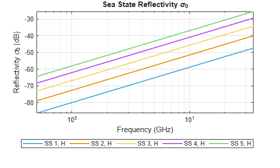
Figure は、海面反射率が周波数に比例することを示しています。さらに、海面状態番号が増加 (粗さの増加に相当) すると、反射率も増加しています。

偏波の影響

次に、偏波が海面反射率に及ぼす影響について考察します。前のセクションと同じグレージング角と周波数スパンを維持します。

pol = 'V'; % Vertical polarization

% Initialize reflectivity output
numFreq = numel(freq);
nrcsV = zeros(numFreq,numSeaStates);

% Calculate reflectivity
for is = 1:numSeaStates
    nrcsV(:,is) = seareflectivity(ss(is),grazAng,freq,'Polarization',pol);
end

% Plot reflectivity
hAxes = helperPlotSeaReflectivity(ss,grazAng,freq,nrcsH,'H');
helperPlotSeaReflectivity(ss,grazAng,freq,nrcsV,'V',hAxes);

Figure は、偏波によって反射率に顕著な影響があることを示している。高周波数よりも低周波数の方が、水平偏波と垂直偏波の差が大きいことに注意してください。海面状態番号が増加するにつれて、水平偏波と垂直偏波の差は減少します。したがって、周波数が高くなるほど、偏波への依存性は減少します。

グレージング角の影響

グレージング角の影響について考察します。L バンド周波数 1.5GHz において、0.1 ～ 60 度のレンジにおける海面反射率を計算します。

grazAng = linspace(0.1,60,100); % Grazing angle (deg)
freq = 1.5e9; % L-band frequency (Hz)

% Initialize reflectivity output
numGrazAng = numel(grazAng);
nrcsH = zeros(numGrazAng,numSeaStates);
nrcsV = zeros(numGrazAng,numSeaStates);

% Calculate reflectivity
for is = 1:numSeaStates
    nrcsH(:,is) = seareflectivity(ss(is),grazAng,freq,'Polarization','H');
    nrcsV(:,is) = seareflectivity(ss(is),grazAng,freq,'Polarization','V');
end

% Plot reflectivity
hAxes = helperPlotSeaReflectivity(ss,grazAng,freq,nrcsH,'H');
helperPlotSeaReflectivity(ss,grazAng,freq,nrcsV,'V',hAxes);
ylim(hAxes,[-60 -10]);

Figure から、グレージング角が小さいほど海面反射率の変動が大きく、垂直偏波と水平偏波の間にも差異が存在することがわかります。Figure は、グレージング角が大きくなるにつれて、グレージング角への依存性が減少することを示しています。さらに、検討したグレージング角のレンジにおいて、同じ海面状態であれば、水平偏波信号の反射率は垂直偏波信号の反射率よりも低くなります。

海上監視レーダーの例

C/N 比の計算

6 GHz (C バンド) で動作する水平偏波の海上監視レーダー システムについて考えます。レーダー システムを定義します。

% Radar parameters 
freq = 6e9;         % C-band frequency (Hz) 
anht = 20;          % Height (m) 
ppow = 200e3;       % Peak power (W)
tau  = 200e-6;      % Pulse width (sec)
prf  = 300;         % PRF (Hz)
azbw = 10;          % Half-power azimuth beamwidth (deg)
elbw = 30;          % Half-power elevation beamwidth (deg)
Gt   = 22;          % Transmit gain (dB) 
Gr   = 10;          % Receive gain (dB)
nf   = 3;           % Noise figure (dB)
Ts   = systemp(nf); % System temperature (K)

次に、海面状態が 2 である運用環境をシミュレーションします。定義されたジオメトリのグレージング角における海面反射率を計算してプロットします。

% Sea parameters
ss = 2;             % Sea state    

% Calculate surface state
[hgtsd,beta0] = searoughness(ss);

% Setup geometry
anht = anht + 2*hgtsd;         % Average height above clutter (m) 
surfht = 3*hgtsd;              % Surface height (m) 

% Calculate maximum range for simulation
Rua = time2range(1/prf); % Maximum unambiguous range (m)
Rhoriz = horizonrange(anht,'SurfaceHeight',surfht); % Horizon range (m)
Rmax = min(Rua,Rhoriz); % Maximum simulation range (m)

% Generate vector of ranges for simulation
Rm = linspace(100,Rmax,1000); % Range (m)
Rkm = Rm*1e-3;                % Range (km) 

% Calculate sea clutter reflectivity. Temporarily permit values outside of
% the NRL sea reflectivity model grazing angle bounds of 0.1 - 60 degrees.
% Specifically, this is to permit analysis of grazing angles less than 0.1
% degrees that are close to the horizon.
grazAng = grazingang(anht,Rm,'TargetHeight',surfht); 
warning('off','radar:radar:outsideValidityRegion'); % Permit values outside model
nrcs = seareflectivity(ss,grazAng,freq);
warning('on','radar:radar:outsideValidityRegion'); % Turn warnings back on
helperPlotSeaReflectivity(ss,grazAng,freq,nrcs,'H');

次に、clutterSurfaceRCS 関数を使用して、クラッターのレーダー断面積 (RCS) を計算します。レーダーの水平線レンジに到達することでクラッター RCS が落ち込んでいることに注目してください。

% Calculate clutter RCS 
rcs = clutterSurfaceRCS(nrcs,Rm,azbw,elbw,grazAng(:),tau); 
rcsdB = pow2db(rcs); % Convert to decibels for plotting
hAxes = helperPlot(Rkm,rcsdB,'RCS','Clutter RCS (dBsm)','Clutter Radar Cross Section (RCS)');
helperAddHorizLine(hAxes,Rhoriz);

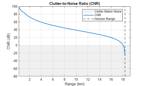
radareqsnr 関数を使用して、C/N 比 (CNR) を計算します。ここでも、シミュレーション レンジがレーダー水平線に近づくにつれて CNR が落ち込んでいることに注目してください。クラッターがノイズを下回るレンジを計算します。

% Convert frequency to wavelength
lambda = freq2wavelen(freq); 

% Calculate and plot the clutter-to-noise ratio
cnr = radareqsnr(lambda,Rm(:),ppow,tau,... 
        'gain',[Gt Gr],'rcs',rcs,'Ts',Ts); % dB
hAxes = helperPlot(Rkm,cnr,'CNR','CNR (dB)','Clutter-to-Noise Ratio (CNR)');
ylim(hAxes,[-80 100]);
helperAddHorizLine(hAxes,Rhoriz);
helperAddBelowClutterPatch(hAxes);

% Range when clutter falls below noise
helperFindClutterBelowNoise(Rkm,cnr);

Range at which clutter falls below noise (km) = 18.04

伝播パスの考慮

レーダーとクラッターの間のパスが自由空間条件から逸脱する場合は、クラッター伝播係数とパス上の大気損失を考慮に入れます。クラッター伝播係数は、radarpropfactor 関数を使用して計算できます。

% Calculate radar propagation factor for clutter 
Fc = radarpropfactor(Rm,freq,anht,surfht, ... 
    'SurfaceHeightStandardDeviation',hgtsd,...
    'SurfaceSlope',beta0,...
    'ElevationBeamwidth',elbw);
helperPlot(Rkm,Fc,'Propagation Factor', ...
    'Propagation Factor (dB)', ...
    'One-Way Clutter Propagation Factor F_C');

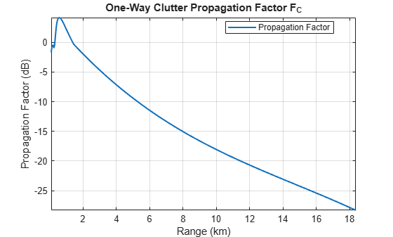
上記のプロットには、次の 2 つの伝播領域が見て取れます。

1. 干渉領域: ここは、反射波が直射波と干渉する領域です。これは、ロービングが発生しているレンジに現れます。

2. 中間領域: これは干渉領域と回折領域の間の領域です。ここで、回折領域は水平線を超えた影の領域として定義されます。この例において、曲線が約 1.5km の地点で折れ曲がる部分で発生する中間領域は、一般的に干渉領域と回折領域の間の内挿によって推定されます。

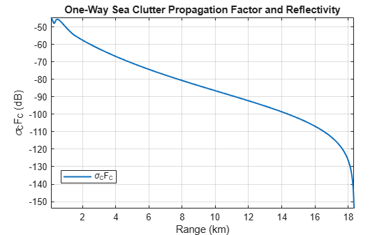
通常、クラッター伝播係数と海面反射率は積 ${\sigma }_C{F}_C^4$ として組み合わせられます。なぜなら、表面反射率の測定値は、通常、反射率 ${\sigma }_C$ 単体ではなく、この積の形で測定されるためです。この積を計算し、結果をプロットします。

% Combine clutter reflectivity and clutter propagation factor
FcLinear = db2mag(Fc); % Convert to linear units
combinedFactor = nrcs.*FcLinear.^2;
combinedFactordB = pow2db(combinedFactor);
helperPlot(Rkm,combinedFactordB,'\sigma_CF_C', ...
    '\sigma_CF_C (dB)', ...
    'One-Way Sea Clutter Propagation Factor and Reflectivity');

次に、傾斜パス用の tropopl 関数を使用して、パス上の大気損失を計算します。計算には、既定の標準大気モデルを使用します。

% Calculate one-way loss associated with atmosphere
elAng = height2el(surfht,anht,Rm); % Elevation angle (deg) 
numEl = numel(elAng);
Latmos = zeros(numEl,1);
for ie = 1:numEl
    Latmos(ie,:) = tropopl(Rm(ie),freq,anht,elAng(ie));
end
helperPlot(Rkm,Latmos,'Atmospheric Loss','Loss (dB)','One-Way Atmospheric Loss');

CNR を再計算します。伝播係数と大気損失を計算に含めます。CNR 曲線の形状の変化に注目してください。これらの要素を考慮に入れると、クラッターがノイズを下回る地点は、より近いレンジに収まります。

% Re-calculate CNR including radar propagation factor and atmospheric loss
cnr = radareqsnr(lambda,Rm(:),ppow,tau,... 
        'gain',[Gt Gr],'rcs',rcs,'Ts',Ts, ...
        'PropagationFactor',Fc,...
        'AtmosphericLoss',Latmos); % dB
helperAddPlot(Rkm,cnr,'CNR + Propagation Factor + Atmospheric Loss',hAxes);

% Range when clutter falls below noise
helperFindClutterBelowNoise(Rkm,cnr);

Range at which clutter falls below noise (km) = 10.44

気象の影響について

大気がターゲットの検出に影響を与えるのと同様に、気象もクラッターの検出に影響を与えます。シミュレーション レンジにおける降雨の影響を考慮します。まず、降雨減衰率を計算します。

% Calculate one-way loss associated with rain
rr = 50;                           % Rain rate (mm/h)
polAng = 0;                        % Polarization tilt angle (0 degrees for horizontal) 
elAng = height2el(surfht,anht,Rm); % Elevation angle (deg) 
numEl = numel(elAng);
Lrain = zeros(numEl,1);
for ie = 1:numEl
    Lrain(ie,:) = cranerainpl(Rm(ie),freq,rr,elAng(ie),polAng);
end
helperPlot(Rkm,Lrain,'Rain Loss','Loss (dB)','One-Way Rain Loss');

CNR を再計算します。伝播パスと降雨損失を含めます。雨が存在することによる CNR の低下はわずかであることに注意してください。

% Re-calculate CNR including radar propagation factor, atmospheric loss,
% and rain loss
cnr = radareqsnr(lambda,Rm(:),ppow,tau,... 
        'gain',[Gt Gr],'rcs',rcs,'Ts',Ts, ...
        'PropagationFactor',Fc, ...
        'AtmosphericLoss',Latmos + Lrain); % dB
helperAddPlot(Rkm,cnr,'CNR + Propagation Factor + Atmospheric Loss + Rain',hAxes);

% Range when clutter falls below noise
helperFindClutterBelowNoise(Rkm,cnr);

Range at which clutter falls below noise (km) = 9.61

まとめ

この例では、海面シミュレーションに関する概念を紹介します。海面反射率は以下の性質を示します。

• 海面状態に対する強い依存性

• 周波数に対する比例的依存性

• 周波数の増加とともに減少する偏波依存性

• 低グレージング角における、グレージング角への強い依存性

この例では、海上監視レーダー システムの C/N 比を計算するために、海面状態の物理的性質と反射率をどのように使用するかについても説明します。さらに、この例では伝播パスのシミュレーションを改善する方法についても説明します。

参考文献

1. Barton, David Knox. Radar Equations for Modern Radar. Artech House Radar Series. Boston, Mass: Artech House, 2013.

2. Blake, L. V. Machine Plotting of Radar Vertical-Plane Coverage Diagrams. NRL Report, 7098, Naval Research Laboratory, 1970.

3. Gregers-Hansen, V., and R. Mittal. An Improved Empirical Model for Radar Sea Clutter Reflectivity. NRL/MR, 5310-12-9346, Naval Research Laboratory, 27 Apr. 2012.

4. Richards, M. A., Jim Scheer, William A. Holm, and William L. Melvin, eds. Principles of Modern Radar. Raleigh, NC: SciTech Pub, 2010.

function helperPlotSeaRoughness(ss,hgtsd,beta0,vw)
% Creates 3x1 plot of sea roughness outputs 

% Create figure
figure

% Plot standard deviation of sea wave height
subplot(3,1,1)
plot(ss,hgtsd,'-o','LineWidth',1.5)
ylabel([sprintf('Wave\nHeight ') '\sigma_h (m)'])
title('Sea Wave Roughness')
grid on; 

% Plot sea wave slope
subplot(3,1,2)
plot(ss,beta0,'-o','LineWidth',1.5)
ylabel([sprintf('Wave\nSlope ') '\beta_0 (deg)'])
grid on; 

% Plot wind velocity 
subplot(3,1,3)
plot(ss,vw,'-o','LineWidth',1.5)
xlabel('Sea State')
ylabel([sprintf('Wind\nVelocity ')  'v_w (m/s)'])
grid on; 
end

function hAxes = helperPlotSeaReflectivity(ss,grazAng,freq,nrcs,pol,hAxes)
% Plot sea reflectivities 

% Create figure and new axes if axes are not passed in
newFigure = false; 
if nargin < 6
    figure();
    hAxes = gca; 
    newFigure = true;
end

% Get polarization string
switch lower(pol)
    case 'h'
        lineStyle = '-';
    otherwise
        lineStyle = '--';
end

% Plot
if numel(grazAng) == 1
    hLine = semilogx(hAxes,freq(:).*1e-9,pow2db(nrcs),lineStyle,'LineWidth',1.5);
    xlabel('Frequency (GHz)')
else
    hLine = plot(hAxes,grazAng(:),pow2db(nrcs),lineStyle,'LineWidth',1.5);
    xlabel('Grazing Angle (deg)')
end

% Set display names
numLines = size(nrcs,2);
for ii = 1:numLines
    hLine(ii).DisplayName = sprintf('SS %d, %s',ss(ii),pol);
    if newFigure
        hLine(ii).Color = brighten(hLine(ii).Color,0.5);
    end
end

% Update labels and axes 
ylabel('Reflectivity \sigma_0 (dB)')
title('Sea State Reflectivity \sigma_0')
grid on
axis tight
hold on; 

% Add legend
legend('Location','southoutside','NumColumns',5,'Orientation','Horizontal');
end

function varargout = helperPlot(Rkm,y,displayName,ylabelStr,titleName)
% Used in CNR analysis

% Create figure 
hFig = figure;
hAxes = axes(hFig); 

% Plot
plot(hAxes,Rkm,y,'LineWidth',1.5,'DisplayName',displayName);
grid(hAxes,'on');
hold(hAxes,'on');
xlabel(hAxes,'Range (km)')
ylabel(hAxes,ylabelStr);
title(hAxes,titleName);
axis(hAxes,'tight');

% Add legend
legend(hAxes,'Location','Best')

% Output axes
if nargout ~= 0 
    varargout{1} = hAxes;
end
end

function helperAddPlot(Rkm,y,displayName,hAxes)
% Used in CNR analysis

% Plot
ylimsIn = get(hAxes,'Ylim');
plot(hAxes,Rkm,y,'LineWidth',1.5,'DisplayName',displayName);
axis(hAxes,'tight');
ylimsNew = get(hAxes,'Ylim');
set(hAxes,'Ylim',[ylimsIn(1) ylimsNew(2)]); 
end

function helperAddHorizLine(hAxes,Rhoriz)
% Add vertical line indicating horizon range

xline(Rhoriz.*1e-3,'--','DisplayName','Horizon Range','LineWidth',1.5);
xlims = get(hAxes,'XLim');
xlim([xlims(1) Rhoriz.*1e-3*(1.05)]);
end

function helperAddBelowClutterPatch(hAxes)
% Add patch indicating when clutter falls below the noise

xlims = get(hAxes,'Xlim');
ylims = get(hAxes,'Ylim');
x = [xlims(1) xlims(1) xlims(2) xlims(2) xlims(1)];
y = [ylims(1) 0 0 ylims(1) ylims(1)];
hP = patch(hAxes,x,y,[0.8 0.8 0.8], ...
    'FaceAlpha',0.3,'EdgeColor','none','DisplayName','Clutter Below Noise');
uistack(hP,'bottom');
end

function helperFindClutterBelowNoise(Rkm,cnr)
% Find the point at which the clutter falls below the noise
idxNotNegInf = ~isinf(cnr); 
Rclutterbelow = interp1(cnr(idxNotNegInf),Rkm(idxNotNegInf),0); 
fprintf('Range at which clutter falls below noise (km) = %.2f\n',Rclutterbelow)
end