Sparse Array Design Using CRLB Optimization

Since R2026a

Introduction

This example demonstrates how to design a sparse array by optimizing the Cramer-Rao Lower Bound (CRLB) for direction-of-arrival (DOA) estimation. Suppose we start with an original array of N elements. Our objective is to select the best K elements that minimize the DOA estimation CRLB. This approach is particularly useful for designing fixed subarrays optimized for a specific angle. Additionally, this method is applicable in radar systems where the number of available RF chains is fewer than the number of antennas. In such cases, dynamically optimizing the array-to-RF chain connections for different scan angles can significantly enhance the DOA estimation accuracy.

Array Configuration

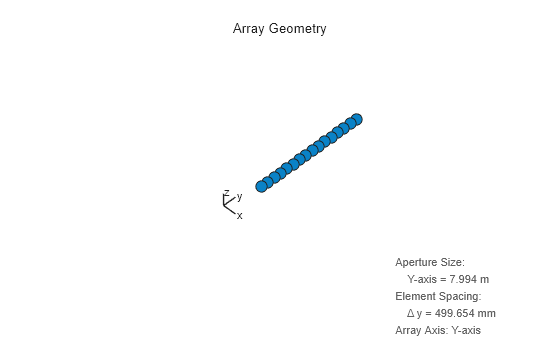
Construct a uniform linear array (ULA) consisting of 16 isotropic antenna elements with half-wavelength element spacing. Visualize this ULA.

% Define system parameters
fc = 300e6;                    % Center frequency
lambda = freq2wavelen(fc);     % Wavelength
N = 16;                        % Number of elements

% Create and visualize ULA
array = phased.ULA(N,lambda/2);
element_pos = getElementPosition(array);
viewArray(array)

Sparse Array Design Via CRLB Minimization

We present a constrained optimization framework for sparse array design that minimizes the CRLB for DOA estimation at a target angle $$\theta$$:

$$\begin{array}{l}\underset{w}{\min }CRL{B}_{\theta }(w)\\ s.t.1^{T}w=K,\\ [w{]}_n\in \{0,1\},n\in \{1,2,\dots ,N\}.\end{array}$$

Problem Components:

1. Objective: Minimize CRLB at angle $$\theta$$

2. Antenna selection vector: Binary vector $$w$$ of length N (1=selected, 0=not selected)

3. Constraint: Exactly K elements must be selected (K < N)

prob = optimproblem(ObjectiveSense = 'min');
w = optimvar('w', N, Type = 'integer', LowerBound = 0, UpperBound = 1);

The objective function $$CRL{B}_{\theta }(w)$$, specified in crlbAntennaSelection, computes the CRLB corresponding to a given antenna selection. The function takes the noise variance and the look direction $$\theta$$ as known inputs, while the antenna selection vector $$w$$ serves as its variable. This setup allows the function to evaluate the CRLB for any specified configuration of selected antennas.

ang = 0;
ncov = 1e-3;
prob.Objective = fcn2optimexpr(@(w) crlbAntennaSelection(element_pos,ang,ncov,w), w);

The crlbAntennaSelection function models the received signal using the steering vector corresponding to the selected sparse array configuration. The noise is assumed to be white Gaussian with a specified variance. The CRLB is then calculated at the given look angle.

function crlb_selected = crlbAntennaSelection(elementPos,ang,ncov,w)
sig = @(ang) steervec(elementPos(:,w == 1),ang);
crlb_selected = crlb(sig, ncov, ang, DataComplexity = 'Complex');
end

Set the number of elements in the sparse array to 8. To enforce this, include a constraint that exactly 8 elements must be selected from the original array.

K = 8;
cons = sum(w) == K;
prob.Constraints.cons = cons;

Display the optimization problem.

show(prob)

  OptimizationProblem : 

	Solve for:
       w
	where:
       w integer
	minimize :
       arg1

       where:

           anonymousFunction1 = @(w)crlbAntennaSelection(element_pos,ang,ncov,w);
           arg1 = anonymousFunction1(w);


	subject to cons:
       w(1) + w(2) + w(3) + w(4) + w(5) + w(6) + w(7) + w(8) + w(9) + w(10) + w(11) + w(12) + w(13) + w(14) + w(15) + w(16) == 8

	variable bounds:
       0 <= w(1)  <= 1
       0 <= w(2)  <= 1
       0 <= w(3)  <= 1
       0 <= w(4)  <= 1
       0 <= w(5)  <= 1
       0 <= w(6)  <= 1
       0 <= w(7)  <= 1
       0 <= w(8)  <= 1
       0 <= w(9)  <= 1
       0 <= w(10) <= 1
       0 <= w(11) <= 1
       0 <= w(12) <= 1
       0 <= w(13) <= 1
       0 <= w(14) <= 1
       0 <= w(15) <= 1
       0 <= w(16) <= 1

init_w = zeros(1,N);
init_w(randperm(N,K)) = 1;
x0.w = init_w;
[sol,fval] = solve(prob,x0);

Solving problem using ga.
ga stopped because the average change in the penalty function value is less than options.FunctionTolerance and 
the constraint violation is less than options.ConstraintTolerance.

Visualize Optimized Sparse Array

Configure a conformal array based on the optimized antenna selection vector. Visualize the resulting sparse array to illustrate the selected antenna positions. The optimized solution reveals that the optimal sparse array places K/2 elements at each end of the original ULA. This arrangement preserves the aperture of the full array, which is critical for achieving the best possible DOA estimation accuracy with the given number of elements.

sparse_element_pos = element_pos(:,sol.w == 1);
sparse_array = phased.ConformalArray(...
    ElementPosition = sparse_element_pos);
viewArray(sparse_array)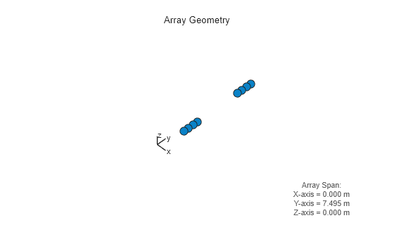

Directivity Pattern Comparison

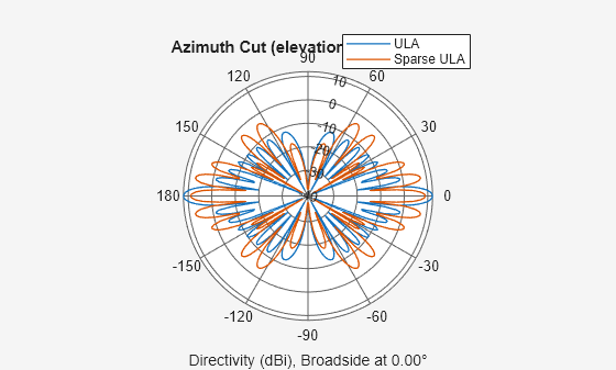
Compare the directivity patterns of the original ULA and the optimized sparse array. This comparison highlights the impact of antenna selection on array performance, illustrating how the sparse configuration affects the main lobe height and sidelobe levels relative to the full array.

fig = figure;
ax = axes;
patternAzimuth(array,fc,Parent=ax)
hold(ax, 'on')
patternAzimuth(sparse_array,fc,Parent=ax)
legend(ax, 'off')
legend(ax, {'ULA','Sparse ULA'})

Further Exploration

To investigate the effects of different array geometries, you can replace phased.ULA with other array system objects available in the Phased Array System Toolbox. This allows you to visualize both the geometries and directivity patterns of optimized sparse arrays for various array configurations.

Reference

[1] A. Atalik, M. Yilmaz and O. Arikan, "Radar Antenna Selection for Direction-of-Arrival Estimations," 2021 IEEE Radar Conference (RadarConf21), Atlanta, GA, USA, 2021, pp. 1-6.