Hardware Array Data Collection and Simulation

Description

In this example, we use an educational hardware phased array platform from Analog Devices, Inc (ADI) to collect real world data and compare with simulated data using the Phased Array System Toolbox.

We first perform a simple calibration routine to set the analog and digital gain and phase of each antenna element and subarray channel. We then compare the pattern of the uncalibrated and calibrated antenna to the ideal pattern predicted by a model of the array using Phased Array System Toolbox.

After calibrating the antenna, we look at the agreement between simulated data and measured data in various situations, such as when certain antenna elements are disabled to create a sparse array, when the antenna pattern is tapered to reduce the sidelobe level, and when a null cancellation technique is implemented for antenna steering.

Setup Description

The hardware setup used is modelled using the Phased Array System Toolbox. The setup consists of a simple isotropic CW transmitter as well as a phased array receiver which is made up of two subarrays, both containing four antenna elements. A picture of the receiver, transmitter, and overall setup are shown below.

Note that each antenna element is comprised of four patch antennas, so what looks like 32 receive antenna elements is actually 32 / 4 = 8 antenna elements.

This wiki page from ADI contains more information on getting the phased array board used for this example up and running.

Transmit Antenna Model

A simple CW transmitter is used to generate the signal measured by the antenna array. A model of the transmitter is created in this section. The pattern of the transmit antenna is estimated as isotropic.

fc = 10.4115e9;
txelement = phased.IsotropicAntennaElement;
radiator = phased.Radiator("Sensor",txelement,"OperatingFrequency",fc);

Receive Antenna Model

A model of the phased array used to collect data for this example is described and constructed in this section. For a detailed schematic of this array, see [1].

The phased array antenna operates in a portion of the X band from 10.0 to 10.5 GHz.

frange = [10.0e9 10.5e9];

Sampling occurs at 30 MHz, 1024 samples are collected for each frame. The Analog to Digital Converter (ADC) is a 12-bit device, so the collected samples have a range of values from -2^11 to 2^11.

sampleRate = 30e6;
nsamples = 1024;
adcbits = 12;
maxdatavalue = 2^(adcbits-1);

Each antenna element in the array is modelled as cosine. Each antenna element channel has a Low Noise Amplifier (LNA), a phase shifter, and an adjustable gain. The default phase shift and gain for each channel are the values that are adjusted during calibration.

element = phased.CosineAntennaElement('FrequencyRange',frange);

The array consists of two subarrays made up of four antenna elements each. The element spacing is half of the shortest wavelength in the frequency range. Use a ULA to model the antenna elements.

lambdaRange = freq2wavelen(frange);
spacing = lambdaRange(2)/2;
nSubarrayElements = 4;
nSubarrays = 2;
array = phased.ULA('Element',element,'NumElements',nSubarrayElements*nSubarrays,'ElementSpacing',spacing);

The ideal receiver is characterized based on the Low Noise Amplifier (LNA) found in the ADI Phaser, the ADL8107 [2]. This LNA has a gain of 24 dB, an output third-order intercept point (OIP3) of 29 dBm, and a Noise figure of 1.3 dB.

receiverGain = 24;
receiverOip3 = 29;
receiverNf = 1.3;
idealReceiver = phased.Receiver(GainMethod="Cubic polynomial",Gain=receiverGain,OIP3=receiverOip3,NoiseMethod="Noise figure",NoiseFigure=receiverNf,SampleRate=sampleRate);

The gain curve for the receiver is demonstrated below.

idealReceiver.viewGain();

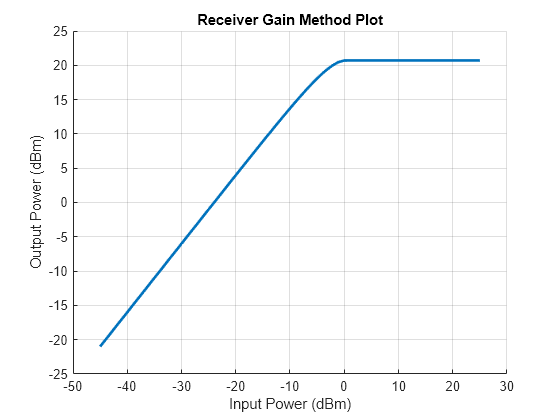
We can see that the non-linear gain region starts at an input power of about -10 dBm, and saturates at about 0 dBm. With the current setup, the amplifier does not saturate. Even if the amplifier were to saturate, there would be limited impact considering the current setup in which a single tone CW waveform is received. The non-linearity of the receiver amplifier would impact performance if the received waveform spanned a wider bandwidth or of the received signal had variable amplitude.

Setup Geometry

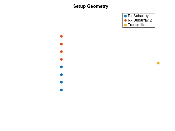
The transmitter is placed at boresight of the receive array. This helper function visualizes the geometry of the setup.

helperVisualizeSetupGeometry(array,nSubarrayElements,spacing);

Simulating Received Signal

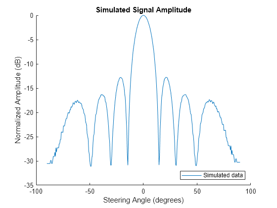
The models created above are used to simulate the expected pattern as the receive array beam is steered from -90 to 90 degrees. This simulated data is used to determine the effectiveness of the calibration routine performed in the following sections. A helper function is used to simulate the received signal. For more information on simulating signal propagation using the Phased Array System Toolbox, see Signal Simulation.

steerangle = -90:0.5:90;
rxamp = helperSimulateAntennaSteering(array,idealReceiver,steerangle,radiator,nsamples,fc,sampleRate);

The plot of the simulated received amplitude with ideal receiver characteristics shows what the data collected on the real system is expected to look like.

rxampdb = mag2db(rxamp);
helperPlotAntennaPattern("Simulated Signal Amplitude",{"Simulated data"},{steerangle},{rxampdb});

Antenna Calibration

Before measuring the beampattern of the antenna array, the phase shifter and gain on each individual element channel as well as the overall amplitude and phase of the two subarray channels are calibrated. Data was collected and included as part of this example to illustrate the calibration routine.

load('CalibrationData.mat','CalibrationData');

Collected Data Format

Before walking through the antenna calibration, it is worth discussing the format of the collected data and how signal amplitude is extracted from the captured data.

The IQ data captured from the receive antenna contains 1024 samples in a frame sampled at 30 MHz as previously discussed. The data is captured independently from each of the two subarrays, so each data snapshot is a 1024x2 matrix of complex numbers.

exampledata = CalibrationData.ExampleData;

The data is sampled at baseband after down-conversion. The data sample values are unitless. The sample amplitude is always considered as a portion of the maximum measurable signal voltage. It is useful to convert the data sample values to a fraction of the maximum possible measured value which is dictated by the number of bits in the ADC.

exampledatascaled = exampledata / maxdatavalue;

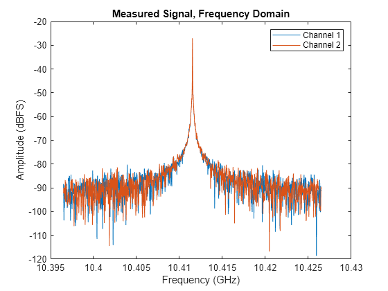
The signal amplitude is extracted by converting to the frequency domain and taking the amplitude of the largest magnitude tone, which is produced by the CW transmitter. The signal amplitude is always expressed in dB Full Scale (dBFS) terms, which indicates the amplitude of the signal compared to the maximum measurable signal for the device in dB.

% Convert the signal to the frequency domain
fexampledata = mag2db(abs(fft(exampledatascaled)) / nsamples);

% Caculate the frequency of the spectrum
fspread = -sampleRate/2:sampleRate/(nsamples-1):sampleRate/2;
frequency = fc + fspread;

% Plot the frequency spectrum of the two channels
ax = axes(figure);
lines = plot(ax,frequency/1e9,fftshift(fexampledata));
lines(1).DisplayName = 'Channel 1'; lines(2).DisplayName = 'Channel 2';
title('Measured Signal, Frequency Domain'); legend();
xlabel('Frequency (GHz)'); ylabel('Amplitude (dBFS)')

% Output the measured signal amplitude
amplitudes = max(fexampledata);
disp(['Channel 1 Amplitude = ',sprintf('%0.1f',amplitudes(1)),' dBFS, Channel 2 Amplitude = ',sprintf('%0.1f',amplitudes(2)),' dBFS']);

Channel 1 Amplitude = -27.1 dBFS, Channel 2 Amplitude = -27.2 dBFS

For the remainder of this example, when signal amplitude is discussed, it is determined using this approach.

Antenna Pattern Data Format

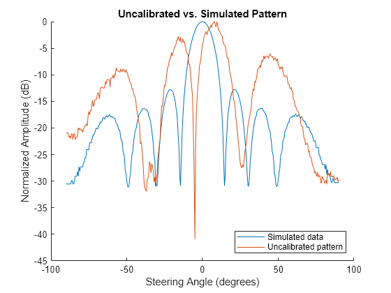
After each calibration step, the antenna pattern is collected by steering the phased array beam from -90 to 90 degrees in 0.5 degree increments with the transmitter placed at 0 degrees and combining the output of the two subarray channels. So the format of the antenna pattern data for this example is a 1024 (number of samples) x 361 (number of steering angles) complex double matrix. To create the antenna pattern plot, the amplitude of the signal at each steering angle is calculated using the process described above. This amplitude extraction has already been performed on the collected data to reduce data size. This amplitude is normalized to 0 dB and plotted against the simulated antenna pattern to illustrate the effects of calibration.

% Get the uncalibrated antenna pattern amplitude
uncalpattern = CalibrationData.AntennaPattern.UncalibratedPattern;

% Plot the actual antenna pattern against the simulated pattern
helperPlotAntennaPattern("Uncalibrated vs. Simulated Pattern",{"Simulated data","Uncalibrated pattern"},{steerangle,steerangle},{rxampdb,uncalpattern});

Analog Calibration

The first part of the calibration routine is calibrating the gain and phase shifter in the analog RF path for each antenna element in the two subarrays. The calibration values that are calculated in this section are used to configure the hardware in the phased array antenna.

Element Course Amplitude Calibration

The first step in the calibration routine is calibrating each element in the subarrays so that their amplitudes are the same. The amplitude of the signal into each antenna element is adjusted by setting the gain in the element RF path.

The signal amplitude in each element channel is measured by turning off all the other elements in the array. The gain of each antenna element is set such that all elements in a subarray have the same signal amplitude.

% Get the data collected during calibration for each subarray
sub1signals = CalibrationData.AnalogAmplitudeCalibration.CourseSubarray1Data;
sub2signals = CalibrationData.AnalogAmplitudeCalibration.CourseSubarray2Data;

% Get the amplitude of the subarray element signals
sub1amplitudes = helperCalculateAmplitude(sub1signals,maxdatavalue);
sub2amplitudes = helperCalculateAmplitude(sub2signals,maxdatavalue);

For each antenna element, 20 data frames are collected for consistency. Take the mean amplitude for each antenna element.

sub1meanamp = reshape(mean(sub1amplitudes),[1 4]);
sub2meanamp = reshape(mean(sub2amplitudes),[1 4]);

The amplitude calibration values for each element are then set so that the amplitude for every element in the array is equal. The gain values must be set based on the element with the minimum signal amplitude, because gain can only be decreased.

sub1gaincal = min(sub1meanamp) - sub1meanamp;
sub2gaincal = min(sub2meanamp) - sub2meanamp;

% Plot element gain calibration settings
helperPlotElementGainCalibration(sub1meanamp,sub1gaincal,sub2meanamp,sub2gaincal);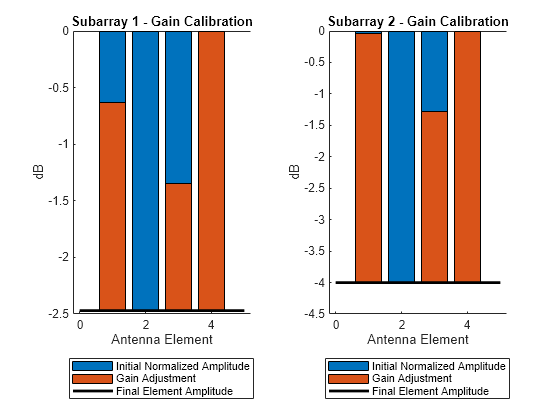

This figure shows that the gain in each element channel is set so that the amplitude of the signal is equal to the amplitude of the signal in the lowest amplitude element for each subarray.

Element Phase Calibration

The phase offset of each element channel varies. Therefore, a default phase offset must be set for each element to align the phase in each element channel.

This phase calibration is performed by turning off all elements in the subarray except for the first element and the element being tested. The phase shift of the first element is left constant at 0 degrees while the phase of the element being tested is shifted from 0 to 360 degrees.

This data is retrieved and the amplitude plotted to illustrate what the results look like.

% Get uncalibrated phased values from calibration data
phasesetting = CalibrationData.AnalogPhaseCalibration.PhaseSetting;
sub1signals = CalibrationData.AnalogPhaseCalibration.Subarray1Measurements;
sub2signals = CalibrationData.AnalogPhaseCalibration.Subarray2Measurements;

% Get the signal amplitudes from 0-360 degree phased offsets for each
% element
sub1amplitudes = helperCalculateAmplitude(sub1signals,maxdatavalue);
sub2amplitudes = helperCalculateAmplitude(sub2signals,maxdatavalue);

% Reshape into a 2d array which is Number Phases x Number Elements
sub1amplitudes = reshape(sub1amplitudes,[numel(phasesetting) 3]);
sub2amplitudes = reshape(sub2amplitudes,[numel(phasesetting) 3]);

% Plot the data
helperPlotPhaseData(phasesetting,sub1amplitudes,sub2amplitudes);

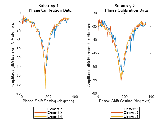
We can see in the plot of the data above that the amplitude of the combined element one and element two signal reaches a minimum at some phase shifter setting. The significance of this minimum is that this is the point at which the actual phase offset between the two channels is 180 degrees.

Based on this data, the phase calibration value is an offset added to the phase shifter setting for each element that ensures that when the phase shift is set to 180 degrees, the true phase shift between elements is actually 180 degrees.

% Calculate the calibration values and display in a table
[~,sub1phaseidx] = min(sub1amplitudes);
[~,sub2phaseidx] = min(sub2amplitudes);
sub1calphase = phasesetting(sub1phaseidx)-180;
sub2calphase = phasesetting(sub2phaseidx)-180;
rowNames = ["Element 1","Element 2","Element 3","Element 4"];
varNames = ["Array 1 calibration phase (deg)","Array 2 calibration phase (deg)"];
t = table([0;sub1calphase'],[0;sub2calphase'],'RowNames',rowNames,'VariableNames',varNames);
disp(t);

                 Array 1 calibration phase (deg)    Array 2 calibration phase (deg)
                 _______________________________    _______________________________

    Element 1                      0                                  0            
    Element 2                 8.4375                             8.4375            
    Element 3                -2.8125                             -5.625            
    Element 4                -2.8125                            -8.4375            

Fine Element Amplitude Calibration

After the initial element phase calibration an additional element amplitude calibration is required. This is due to the impact that phase shifter changes can have on the measured amplitude. The process used for this second analog amplitude calibration is exactly the same as the initial amplitude calibration, so the steps are not repeated here.

The pattern before and after individual element calibration is plotted below.

% Plot the antenna pattern after analog calibration
analogpatterndata = CalibrationData.AntennaPattern.AnalogFineAmplitudeCalPattern;
helperPlotAntennaPattern("After Individual Element Calibration",{"Simulated data","Uncalibrated Pattern","Individual Element Calibration"},{steerangle,steerangle,steerangle},{rxampdb,uncalpattern,analogpatterndata})

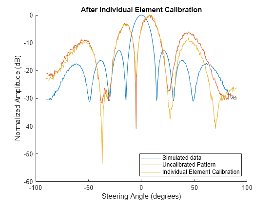
The pattern nulls have gotten deeper after calibrating the element amplitudes and phases. However, the pattern still does not match the simulated antenna pattern due to the phase and amplitude mismatch between the two digital channels. Therefore, an additional digital calibration to align the two subarray channels is required.

Digital Calibration

After the analog calibration steps have been performed for each antenna element, calibration values for the two digital subarray channels are collected so that their amplitudes are equal and the phases align. Unlike the analog calibration, the calibration values calculated in this section are applied to the digital data streams after data collection.

Digital Amplitude Calibration

To calibrate the subarray channel amplitude, the signal in both channels is measured. The amplitude of each signal is determined. The difference is the channel amplitude calibration factor.

% Get the received signal before channel amplitude calibration
digitalrxdata = CalibrationData.DigitalCalibration.MeasuredData;
rxsubarray1 = digitalrxdata(:,1);
rxsubarray2 = digitalrxdata(:,2);

% Calculate amplitude for each subarray
sub1amplitude = helperCalculateAmplitude(rxsubarray1,maxdatavalue);
sub2amplitude = helperCalculateAmplitude(rxsubarray2,maxdatavalue);

% The channel gain offset is the difference in amplitude between channels
channel2GainOffset = sub1amplitude - sub2amplitude

channel2GainOffset = 
-1.2146

Digital Phase Calibration

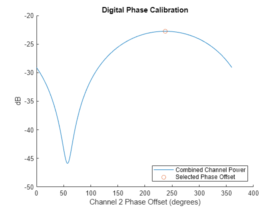
To calibrate the subarray channel phase, the signal in channel 2 is phase shifted from 0 to 360 degrees and combined with the signal in channel 1. When the phases of the two channels have an actual offset of 0 degrees, the amplitude of the combined signals will reach a maximum. The phase offset of channel 2 that results in an actual phase offset of 0 degrees is the digital phase calibration value.

% Phase shift channel 2 from 0 to 360 and combine
phasedeg = 0:360;
phase = deg2rad(phasedeg);
st_vec = [ones(size(phase)); exp(1i*phase)];
combinedsignal = digitalrxdata*conj(st_vec);
combinedamp = helperCalculateAmplitude(combinedsignal,maxdatavalue);
[maxamp, phaseidx] = max(combinedamp);
channel2PhaseOffset = phasedeg(phaseidx);

% Plot the digital phase offset pattern and calibration value
ax = axes(figure); hold(ax,"on");
title(ax,"Digital Phase Calibration"); ylabel(ax,"dB"); xlabel(ax,"Channel 2 Phase Offset (degrees)");
plot(ax,phasedeg,combinedamp,"DisplayName","Combined Channel Power");
scatter(ax,channel2PhaseOffset,maxamp,"DisplayName","Selected Phase Offset");
legend('location','southeast');

Fully Calibrated Antenna Pattern

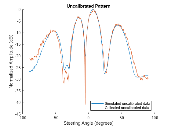
First, we can see how the uncalibrated pattern that was collected compares to the simulated pattern by creating a receiver with same gain and phase errors in each channel that were determined during calibration.

% Get the gains that exist in the array channels - this includes
% differences from the analog and digital channels
channelAbsoluteGains = [sub1meanamp,sub2meanamp-channel2GainOffset];
channelRelativeGains = channelAbsoluteGains - max(channelAbsoluteGains);
channelGains = receiverGain + channelRelativeGains;

% Get the phase offsets that exist in the array channels - this includes
% offsets from the analog and digital channels
channelPhaseOffsets = [0,sub1calphase,[0,sub2calphase]-channel2PhaseOffset];

% Set up the receiver with the gains and phase offsets determined during
% the calibration
uncalibratedReceiver = phased.Receiver(GainMethod="Cubic polynomial",Gain=channelGains,OIP3=receiverOip3,NoiseMethod="Noise figure",NoiseFigure=receiverNf,SampleRate=sampleRate,PhaseOffset=channelPhaseOffsets);

% Get the simulated antenna pattern with the known phase and gain
% errors
uncalsim = helperSimulateAntennaSteering(array,uncalibratedReceiver,steerangle,radiator,nsamples,fc,sampleRate);
uncalsimdb = mag2db(uncalsim);
helperPlotAntennaPattern("Uncalibrated Pattern",{"Simulated uncalibrated data","Collected uncalibrated data"},{steerangle,steerangle},{uncalsimdb,uncalpattern});

Finally, the pattern of the fully calibrated pattern is plotted compared to the simulated pattern.

% Plot the antenna pattern after digital channel amplitude calibration
calpattern = CalibrationData.AntennaPattern.FullCalibration;
helperPlotAntennaPattern("Fully Calibrated Antenna",{"Simulated data","Full Calibration"},{steerangle,steerangle},{rxampdb,calpattern})

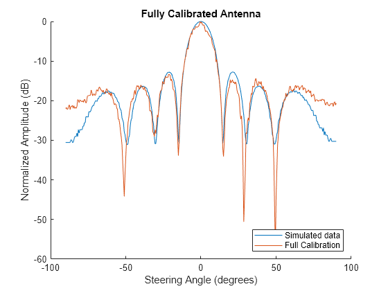
With this final calibration step, the measured antenna pattern closely matches the simulated pattern.

Real Data vs. Simulation

Once calibrated, real data was collected for a few different situations that were also simulated using the Phased Array System Toolbox. This section illustrates that although the simulation predictions are not perfect, they closely match the real data under a number of different operating conditions.

Sparse Array Grating Lobes

Phased arrays can be configured to have spacing between elements of greater than 1/2 wavelength to reduce hardware costs while still meeting functional requirements for the specified task. These sparse arrays will have grating lobes in the array response. The Phased Array System Toolbox can be used to model the array response of any array geometry, including sparse arrays.

In this section, we implemented array sparsity by disabling certain elements in the hardware antenna and capturing beam pattern data. This collected data is compared against simulated data to illustrate the usefulness of the Phased Array System Toolbox in simulating any type of array geometry.

load('SparseArray.mat','SparseArray');

The impairment data contains information about the element that was disabled and the resulting beam pattern that was collected. For the sake of this example, the same antenna element was disabled in both subarrays.

A helper function is used to run a simulation disabling the same elements that were disabled during data collection and comparing the simulated data to the collected data. This data shows that simulation can be used to effectively model the grating lobes introduced by a sparse array.

helperPlotSparseArray(SparseArray,array,idealReceiver,radiator,nsamples,fc,sampleRate);

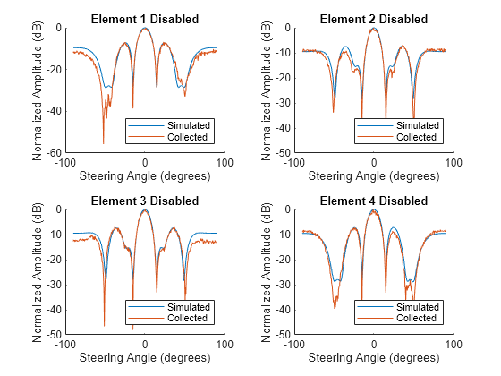
The simulated pattern closely matches the measured pattern when disabling the elements within the subarray.

Tapering

The sidelobe characteristics of a phased array can be altered by attenuating the signal into certain elements in the array. This is a technique known as tapering. Tapering was implemented in the phased array hardware and the measured results were compared to simulation. A Taylor window taper was used in the data collection and simulation. For more information on antenna tapering, see Tapering, Thinning and Arrays with Different Sensor Patterns.

load('AntennaTaperData.mat','AntennaTaperData');

A helper function is used to parse the data and compare with simulated results.

helperPlotAntennaTaper(AntennaTaperData,array,idealReceiver,radiator,nsamples,fc,sampleRate);

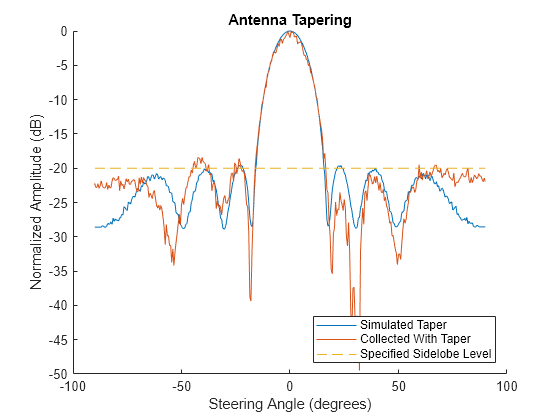
In this case, the results match somewhat closely but the sidelobes are not reduced to the desired extent in the actual hardware implementation.

Pattern Nulling

Nulling is a technique that can be used to avoid the impact of inference on array performance. By inserting a null into the beampattern, the received power from known interferers can be reduced. In this case a simple null cancellation technique is used to null a certain portion of the array pattern. For more information on nulling techniques, see Array Pattern Synthesis Part I: Nulling, Windowing, and Thinning.

load('NullSteeringData.mat','NullSteeringData');

A helper function is used to display the collected data with and without a null in the pattern.

helperNullSteering(NullSteeringData,array,idealReceiver,radiator,nsamples,fc,sampleRate);

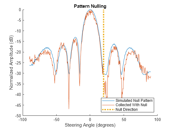
The collected null pattern closely matches the shape of the simulated null pattern.

Summary

In this example we collected data using a real phased array antenna. We walk through a simple calibration routine and show the impact that calibration has on the antenna pattern by comparing the data measured using an uncalibrated and calibrated antenna.

Additionally, we compare the data collected with certain elements disabled, the array pattern tapered, and a null canceller applied to the beam pattern. The Phase Array System Toolbox is used to simulate these various data collection scenarios and the agreement between real world data and simulated data is demonstrated.

Although the simulated data closely matches the collected data in all these scenarios, the fidelity of the model could always be further improved for better results. For example, some areas that could be explored for further model improvements are:

• Add the antenna element patterns for the transmit and receive antennas in place of the isotropic assumption.

• Add environmental noise

• Add impairments such as phase noise and mutual coupling

The level of fidelity required is use case dependent, but even a simple model like the one used in this example provides results that appear very similar to data collected using a real world antenna.

References

[1] Phased Array Radar Workshop. Analog Devices, June 20, 2022, https://www.analog.com/media/en/other/tradeshows/ims2022-adi-phasedarrayworkshop.pdf.

[2] Analog Device Inc. ADL 8107 Low Noise Amplifier, October 16, 2023, https://www.mouser.com/new/analog-devices/adi-adl8107-amplifiers/?gclid=CjwKCAjwvrOpBhBdEiwAR58-3Ds7tNIbmYqhkB-KLX9Ffczui8g1PY0TU5NY16gfMl7Qn0pZN3cwHhoCkC8QAvD_BwE.

Helper Functions

The following helper functions create the visualizations for this example.

function amplitude = helperCalculateAmplitude(data,maxvalue)
    % Get the signal amplitude

    % Scale data
    datascaled = data / maxvalue;
    [nsamples,~] = size(data);

    % Convert the signal to the frequency domain
    fexampledata = mag2db(abs(fft(datascaled)) / nsamples);

    % Amplitude is the largest frequency value
    amplitude = max(fexampledata);
end

function helperPlotAntennaPattern(plottitle,name,steerangle,rxamp,ax)
    % Plot an antenna pattern
    
    % Set up the figure
    if nargin < 5
        ax = axes(figure);
    end
    
    hold(ax,"on"); title(ax,plottitle);
    xlabel(ax,"Steering Angle (degrees)"); ylabel(ax,"Normalized Amplitude (dB)");

    % Plot each antenna pattern that was passed in
    numfigures = numel(name);
    for iFig = 1:numfigures
        curname = name{iFig};
        cursteerangle = steerangle{iFig};
        currxamp = rxamp{iFig};
        plotSinglePattern(ax,curname,cursteerangle,currxamp);
    end

    legend(ax,"location","southeast");

    function plotSinglePattern(ax,name,angle,amp)
        normData = amp - max(amp);
        plot(ax,angle,normData,"DisplayName",name);
    end
    
end

function helperVisualizeSetupGeometry(array,subarrayElements,spacing)
    % Visualize the hardware setup for this example.

    % Setup figure
    f = figure; a = axes(f,"XTick",[],"YTick",[]); a.XAxis.Visible = false; a.YAxis.Visible = false;
    title(a,"Setup Geometry"); hold(a,"on");

    % Get the position of the arrays
    rxArrayPositions = array.getElementPosition();
    subarray1Position = rxArrayPositions(1:2,1:subarrayElements);
    subarray2Position = rxArrayPositions(1:2,subarrayElements+1:end);
    txPosition = [spacing*5;0];

    % Plot the arrays
    scatter(a,subarray1Position(1,:),subarray1Position(2,:),40,"filled","o","MarkerFaceColor",[0,0.44,0.74],"DisplayName","Rx Subarray 1");
    scatter(a,subarray2Position(1,:),subarray2Position(2,:),40,"filled","o","MarkerFaceColor",[0.85,0.32,0.10],"DisplayName","Rx Subarray 2");
    scatter(a,txPosition(1),txPosition(2),40,"yellow","filled","o","MarkerFaceColor",[0.93,0.69,0.12],"DisplayName","Transmitter");
    legend(a); xlim(a,[-spacing*2 txPosition(1)]); ylim(a,[-0.1 0.1]); hold(a,"off");
end

function [array1gaincal,array2gaincal] = helperPlotElementGainCalibration(sub1meanamp,sub1gaincal,sub2meanamp,sub2gaincal)
    % Calculate and visualize the element-wise amplitude calibration for
    % both subarrays.
    
    % Setup figure
    figure; tiledlayout(1,2); a = nexttile();

    % Calculate and plot the gain calibration for subarray 1
    array1gaincal = helperElementSubarrayGainCalibration(a,'Subarray 1',sub1meanamp, sub1gaincal); a = nexttile();
    
    % Calculate and plot the gain calibration for subarray 2
    array2gaincal = helperElementSubarrayGainCalibration(a, 'Subarray 2', sub2meanamp, sub2gaincal);
end

function arraygaincal = helperElementSubarrayGainCalibration(ax,name,amplitudes,arraygaincal)
    % Calculate and visualize the element-wise amplitude calibration for
    % one subarray.

    hold(ax,"on");

    % Normalize amplitude for each element in the array
    dbNormAmplitudes = amplitudes - max(amplitudes);
    
    % Plot normalized amplitudes and gain adjustments
    b = bar(ax,[dbNormAmplitudes',arraygaincal'],'stacked');
    b(1).DisplayName = "Initial Normalized Amplitude";
    b(2).DisplayName = "Gain Adjustment";

    % Plot a line showing the final amplitude of all elements
    plot(ax,[0,5],[min(dbNormAmplitudes),min(dbNormAmplitudes)],"DisplayName","Final Element Amplitude","LineWidth",2,"Color","k")

    xlabel('Antenna Element')
    ylabel('dB');
    title([name ' - Gain Calibration'])
    legend('Location','southoutside')
end

function helperPlotPhaseData(phasesetting,sub1amplitudes,sub2amplitudes)
    % Visualize the element-wise phase calibration data for the entire
    % array.
    figure; tiledlayout(1,2); nexttile();
    helperPlotPhaseSubarrayData("Subarray 1",phasesetting,sub1amplitudes); nexttile();
    helperPlotPhaseSubarrayData("Subarray 2",phasesetting,sub2amplitudes);
end

function helperPlotPhaseSubarrayData(name, phasesetting, phaseOffsetAmplDb)
    % Visualize the element-wise phase calibration data for a subarray.
    lines = plot(phasesetting, phaseOffsetAmplDb);
    lines(1).DisplayName = "Element 2";
    lines(2).DisplayName = "Element 3";
    lines(3).DisplayName = "Element 4";
    title([name,' - Phase Calibration Data'])
    ylabel("Amplitude (dB) Element X + Element 1")
    xlabel("Phase Shift Setting (degrees)")
    legend("Location","southoutside")
end

function helperPlotSparseArray(SparseArrayData,array,receiver,radiator,nsamples,fctransmit,sampleRate)
    % Plot the simulated impairment data as well as the collected
    % impairment data.
    [~,numdisabledelements] = size(SparseArrayData);

    % Setup a tiled figure
    f = figure; tiledlayout(f,2,2);
    
    % Loop through each disabled element. Compare simulation to
    % measurement.
    for iImpair = 1:numdisabledelements

        % Get the element to disable.
        disabledElement = SparseArrayData(iImpair).Element;

        % Get the steer angles to simulate
        steerangle = SparseArrayData(iImpair).SteerAngle;
    
        % Generate the antenna pattern by inserting zeros into disabled
        % elements for analog weights.
        analogweights = ones(4,2);
        analogweights(iImpair,:) = 0;
        rxamp = helperSimulateAntennaSteering(array,receiver,steerangle,radiator,nsamples,fctransmit,sampleRate,analogweights);
        rxampsim = mag2db(rxamp);
        
        % Get the collected antenna pattern
        rxampcollected = SparseArrayData(iImpair).Pattern;
    
        % Plot the figure
        ax = nexttile();
        helperPlotAntennaPattern(['Element ',num2str(disabledElement),' Disabled'],{"Simulated","Collected"},{steerangle,steerangle},{rxampsim,rxampcollected},ax)
    end
end

function helperPlotAntennaTaper(TaperData,array,receiver,radiator,nsamples,fctransmit,sampleRate)
    % Plot the simulated taper pattern as well as the collected
    % impairment data.

    % Get steer angles used
    steerangle = TaperData.SteerAngles;

    % Get the sidelobe level specified
    sidelobelevel = TaperData.SidelobeLevel;
    
    % Get the collected data after tapering
    rxamptaper = TaperData.TaperedPattern;

    % Simulate the antenna pattern using the taper applied during data
    % collection
    analogweights = TaperData.Taper;
    rxdatasim = helperSimulateAntennaSteering(array,receiver,steerangle,radiator,nsamples,fctransmit,sampleRate,analogweights);
    rxampsim = mag2db(rxdatasim);

    % Plot collected data with and without taper as well as simulated taper
    ax = axes(figure);
    helperPlotAntennaPattern("Antenna Tapering",{"Simulated Taper","Collected With Taper"},{steerangle,steerangle},{rxampsim,rxamptaper},ax)
    plot(ax,[steerangle(1),steerangle(end)],[sidelobelevel,sidelobelevel],"DisplayName","Specified Sidelobe Level","LineStyle","--");
end

function helperNullSteering(NullSteeringData,array,receiver,radiator,nsamples,fctransmit,sampleRate)
    % Plot the simulated and collected null steering data

     % Get steer angles used
    steerangle = NullSteeringData.SteerAngles;

    % Get the null angle specified
    nullangle = NullSteeringData.NullAngle;
    
    % Get the collected data after inserting a null
    rxampnull = NullSteeringData.PatternAfterNull;

    % Simulate the antenna pattern with nulling
    rxdatasim = helperSimulateAntennaSteering(array,receiver,steerangle,radiator,nsamples,fctransmit,sampleRate,ones(4,2),ones(2,1),nullangle);
    rxampsim = mag2db(rxdatasim);

    % Plot collected data with and without null as well as simulated null
    ax = axes(figure);
    helperPlotAntennaPattern("Pattern Nulling",{"Simulated Null Pattern","Collected With Null"},{steerangle,steerangle},{rxampsim,rxampnull},ax)
    
    % plot the null location
    rxampsimnorm = rxampsim-max(rxampsim); collectampnorm = rxampnull-max(rxampnull);
    rxampsimnorm(rxampsimnorm == -Inf) = []; collectampnorm(collectampnorm == -Inf) = [];
    minnorm = min([rxampsimnorm,collectampnorm]);
    plot(ax,[nullangle,nullangle],[minnorm,0],"DisplayName","Null Direction","LineStyle",":","LineWidth",3);
end

function [rxamp,rxphase] = helperSimulateAntennaSteering(array,receiver,steerangle,radiator,nsamples,fctransmit,sampleRate,analogweight,digitalweight,nullangle)
    % Simulate antenna steering.
    arguments
        array
        receiver
        steerangle
        radiator
        nsamples
        fctransmit
        sampleRate
        analogweight (4,2) double = ones(4,2)
        digitalweight (2,1) double = ones(2,1)
        nullangle = []
    end

    % Setup collector
    collector = phased.Collector("Sensor",array,"OperatingFrequency",fctransmit,"WeightsInputPort",true);

    % Single tone CW signal is used
    signal = 1e-2*ones(nsamples,1);
    
    % Set up a channel for radiating signal
    channel = phased.FreeSpace("OperatingFrequency",fctransmit,"SampleRate",sampleRate);
    
    % Setup geometry
    rxpos = [0;0;0];
    rxvel = [0;0;0];
    txpos = [0;10;0];
    txvel = [0;0;0];
    [~,ang] = rangeangle(rxpos,txpos);
    
    % Radiate signal
    sigtx = radiator(signal,ang);
    
    % Propagate signal
    sigtx = channel(sigtx,txpos,rxpos,txvel,rxvel);
    
    % Create a beamformer
    psbits = 8;
    directions = [steerangle;zeros(1,length(steerangle))];
    beamformer = phased.PhaseShiftBeamformer("SensorArray",array,"OperatingFrequency",fctransmit,"Direction",directions,"NumPhaseShifterBits",psbits);

    % Create the array weights
    weights = [analogweight(:,1)*digitalweight(1);analogweight(:,2)*digitalweight(2)];

    % Insert a null if a null angle was passed in
    if ~isempty(nullangle)
        % Null the replicated array
        pos = array.getElementPosition() / freq2wavelen(fctransmit);
        null = [nullangle;0];
        nullweight = steervec(pos,null,psbits);
        weights = getNullSteer(weights,nullweight);
    end

    % Collect the signal
    sigcollect = collector(sigtx,[0;0],weights);
    
    % Pass through the receiver
    sigreceive = receiver(sigcollect);

    % Beamform the signal
    sigdigital = beamformer(sigreceive);
    
    % Get the received signal amplitude and phase
    rxphase = mean(rad2deg(angle(sigdigital)),1);
    rxamp = mean(abs(sigdigital),1);
    
    function nullsteer = getNullSteer(steerweight,nullweight)
        rn = nullweight'*steerweight/(nullweight'*nullweight);
        nullsteer = steerweight-nullweight*rn;
    end
end