Specify Coefficients in PDE Modeler App
Coefficients for Scalar PDEs
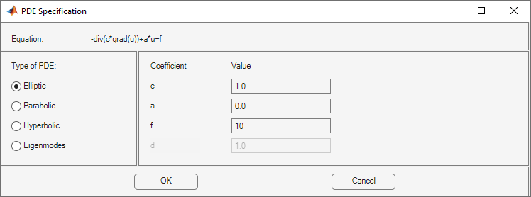
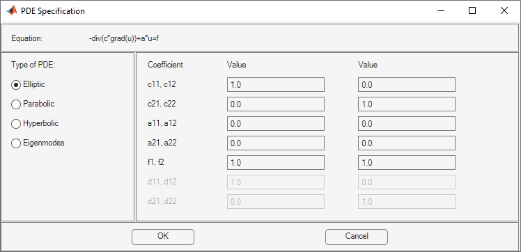
To enter coefficients for your PDE, select PDE > PDE Specification.
Enter text expressions using these conventions:
x— x-coordinatey— y-coordinateu— Solution of equationux— Derivative of u in the x-directionuy— Derivative of u in the y-directiont— Time (parabolic and hyperbolic equations)sd— Subdomain number
For example, you could use this expression to represent a coefficient:
(x + y)./(x.^2 + y.^2 + 1) + 3 + sin(t)./(1 + u.^4)
For elliptic problems, when you include u, ux,
or uy, you must use the nonlinear solver. Select Solve >
Parameters > Use nonlinear solver.
Note
Do not use quotes or unnecessary spaces in your entries. The parser can misinterpret a space as a vector separator, as when a MATLAB® vector uses a space to separate elements of a vector.
Use
.*,./, and.^for multiplication, division, and exponentiation operations. The text expressions operate on row vectors, so the operations must make sense for row vectors. The row vectors are the values at the triangle centroids in the mesh.
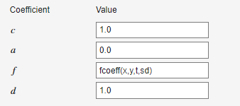
You can write MATLAB functions for coefficients as well as plain text expressions. For example,
suppose your coefficient f is given by the file
fcoeff.m.
function f = fcoeff(x,y,t,sd)

f = (x.*y)./(1 + x.^2 + y.^2); % f on subdomain 1
f = f + log(1 + t); % include time
r = (sd == 2); % subdomain 2
f2 = cos(x + y); % coefficient on subdomain 2
f(r) = f2(r); % f on subdomain 2
Use fcoeff(x,y,t,sd) as the f coefficient in
the parabolic solver.
The coefficient c is a 2-by-2 matrix. You can give 1-, 2-, 3-, or 4-element matrix expressions. Separate the expressions for elements by spaces. These expressions mean:
1-element expression:
2-element expression:
3-element expression:
4-element expression:
For example, c is a symmetric matrix with constant diagonal entries
and cos(xy) as the off-diagonal terms:
1.1 cos(x.*y) 5.5 | (1) |
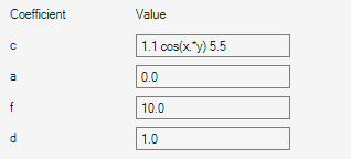
This corresponds to coefficients for the parabolic equation
Coefficients for Systems of PDEs
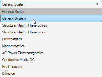
You can enter coefficients for a system with N =
2 equations in the PDE Modeler app. To do so, open the PDE
Modeler app and select Generic System.
Then select PDE > PDE Specification.
Enter character expressions for coefficients using the form in Coefficients for Scalar PDEs, with additional options for nonlinear equations. The additional options are:
Represent the
ith component of the solutionuusing'u(i)'fori= 1 or 2.Similarly, represent the
ith components of the gradients of the solutionuusing'ux(i)'and'uy(i)'fori= 1 or 2.
Note
For elliptic problems, when you include coefficients u(i),
ux(i), or uy(i), you must use the
nonlinear solver. Select Solve > Parameters > Use nonlinear solver.
Do not use quotes or unnecessary spaces in your entries.
For higher-dimensional systems, do not use the PDE Modeler app. Represent your problem coefficients at the command line.
You can enter scalars into the c matrix, corresponding to these
equations:
If you need matrix versions of any of the cij coefficients, enter
expressions separated by spaces. You can give 1-, 2-, 3-, or 4-element matrix
expressions. These mean:
1-element expression:
2-element expression:
3-element expression:
4-element expression:
For example, these expressions show one of each type (1-, 2-, 3-, and 4-element expressions)
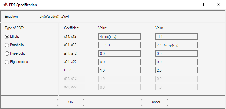
These expressions correspond to the equations
Coefficients That Depend on Time and Space
This example shows how to enter time- and coordinate-dependent coefficients in the PDE Modeler app.
Solve the parabolic PDE,
with the following coefficients:
d = 5
a = 0
f is a linear ramp up to 10, holds at 10, then ramps back down to 0:
c = 1 +.x2 + y2
To solve this equation in the PDE Modeler app, follow these steps:
Write the file
framp.mand save it on your MATLAB path.function f = framp(t) if t <= 0.1 f = 10*t; elseif t <= 0.9 f = 1; else f = 10-10*t; end f = 10*f;
Open the PDE Modeler app by using the
pdeModelercommand.Display grid lines by selecting Options > Grid.
Align new shapes to the grid lines by selecting Options > Snap.
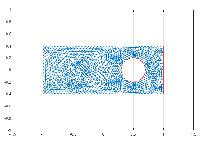
Draw a rectangle with the corners at (-1,-0.4), (-1,0.4), (1,0.4), and (1,-0.4). To do this, first click the
 button. Then click one of the corners using the left mouse
button and drag to draw a rectangle.
button. Then click one of the corners using the left mouse
button and drag to draw a rectangle.Draw a circle with the radius 0.2 and the center at (0.5,0). To do this, first click the
 button. Then right-click the origin and drag to draw a
circle. Right-clicking constrains the shape you draw so that it is a circle
rather than an ellipse. If the circle is not a perfect unit circle, double-click
it. In the resulting dialog box, specify the exact center location and radius of
the circle.
button. Then right-click the origin and drag to draw a
circle. Right-clicking constrains the shape you draw so that it is a circle
rather than an ellipse. If the circle is not a perfect unit circle, double-click
it. In the resulting dialog box, specify the exact center location and radius of
the circle.Model the geometry by entering
R1-C1in the Set formula field.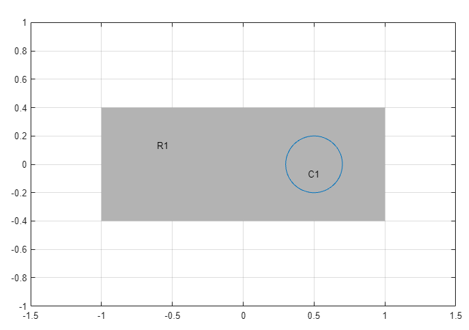
Check that the application mode is set to Generic Scalar.
Specify the boundary conditions. To do this, switch to the boundary mode by selecting Boundary > Boundary Mode. Use Shift+click to select several boundaries. Then select Boundary > Specify Boundary Conditions.
For the rectangle, use the Dirichlet boundary condition with
h = 1andr = t*(x-y).For the circle, use the Neumann boundary condition with
g = x.^2+y.^2andq = 1.
Specify the coefficients by selecting PDE > PDE Specification or clicking the
 button on the toolbar. Select the
Parabolic type of PDE. Specify
button on the toolbar. Select the
Parabolic type of PDE. Specify c = 1+x.^2+y.^2,a = 0,f = framp(t), andd = 5.Note
Do not include quotes or spaces when you specify your coefficients the PDE Modeler app. The parser interprets all inputs as vectors of characters. It can misinterpret a space as a vector separator, as when a MATLAB vector uses a space to separate elements of a vector.
Initialize the mesh by selecting Mesh > Initialize Mesh.
Refine the mesh twice by selecting Mesh > Refine Mesh.
Improve the triangle quality by selecting Mesh > Jiggle Mesh.
Set the initial value and the solution time. To do this, select Solve > Parameters.
In the resulting dialog box, set the time to
linspace(0,1,50)and the initial value u(t0) to0.Solve the equation by selecting Solve > Solve PDE or clicking the
 button on the toolbar.
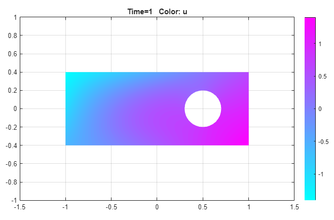
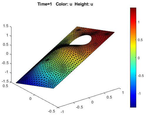
Visualize the solution as a 3-D static plot. To do this:
Select Plot > Parameters.
In the resulting dialog box, select the Color and Height (3-D plot) options.
Select the Show mesh option.
Change the colormap to
jetby using the corresponding drop-down menu in the same dialog box.