Poisson’s Equation with Complex 2-D Geometry: PDE Modeler App

This example shows how to solve the Poisson's equation, –Δu = f on a 2-D geometry created as a combination of two rectangles and two circles.

To solve this problem in the PDE Modeler app, follow these steps:

1. Open the PDE Modeler app by using the pdeModeler command.

2. Display grid lines. To do this, select Options > Grid Spacing and clear the Auto checkbox for the x-axis linear spacing. Enter X-axis linear spacing as -1.5:0.25:1.5. Then select Options > Grid.

3. Align new shapes to the grid lines by selecting Options > Snap.

4. Draw two circles: one with the radius 0.4 and the center at (-0.5,0) and another with the radius 0.2 and the center at (0.5,0.2). To draw a circle, first click the button. Then right-click the origin and drag to draw a circle. Right-clicking constrains the shape you draw so that it is a circle rather than an ellipse.

5. Draw two rectangles: one with corners (-1,0.2), (1,0.2), (1,-0.2), and (-1,-0.2) and another with corners (0.5,1), (1,1), (1,-0.6), and (0.5,-0.6). To draw a rectangle, first click the button. Then click any corner and drag to draw the rectangle.

6. Model the geometry by entering (R1+C1+R2)-C2 in the Set formula field.

7. Save the model to a file by selecting FileSave As.

8. Remove the subdomain borders. To do this, switch to the boundary mode by selecting Boundary > Boundary Mode. Then select Boundary > Remove All Subdomain Borders.

9. Specify the boundary conditions for all circle arcs. Using Shift+click, select these borders. Then select Boundary > Specify Boundary Conditions and specify the Neumann boundary condition with g = -5 and q = 0. This boundary condition means that the solution has a slope of –5 in the normal direction for these boundary segments.

10. For all other boundaries, keep the default Dirichlet boundary condition: h = 1, r = 0.

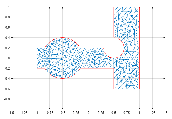
11. Specify the coefficients by selecting PDE > PDE Specification or clicking the PDE button on the toolbar. Specify c = 1, a = 0, and f = 10.

12. Initialize the mesh by selecting Mesh > Initialize Mesh. Refine the mesh by selecting Mesh > Refine Mesh.

    

13. Solve the PDE by selecting Solve > Solve PDE or clicking the = button on the toolbar. The toolbox assembles the PDE problem, solves it, and plots the solution.

    

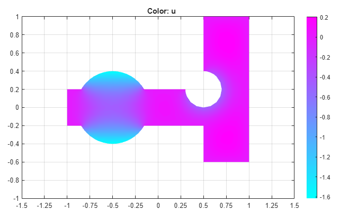
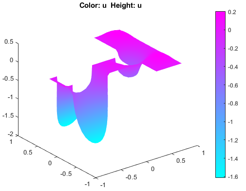
14. Plot the solution as a 3-D plot:

    1. Select Plot > Parameters.

    2. In the resulting dialog box, select Height (3-D plot).

    3. Click Plot.