L-Shaped Membrane with Rounded Corner: PDE Modeler App

This example shows how to compute all eigenvalues smaller than 100 and their corresponding eigenvectors. Consider the eigenvalue problem

–Δu = λu

on an L-shaped membrane with a rounded inner corner. The boundary condition is the Dirichlet condition u = 0.

To solve this problem in the PDE Modeler app, follow these steps:

1. Draw an L-shaped membrane as a polygon with the corners (0,0), (–1,0), (–1,–1), (1,–1), (1,1), and (0,1) by using the pdepoly function.

   pdepoly([0 -1 -1 1 1 0],[0 0 -1 -1 1 1])

2. Draw a circle and a square as follows.

   pdecirc(-0.5,0.5,0.5,'C1') 
   pderect([-0.5 0 0.5 0],'SQ1')

3. Model the geometry with the rounded corner by entering P1+SQ1-C1 in the Set formula field.

4. Check that the application mode is set to Generic Scalar.

5. Remove unnecessary subdomain borders by selecting Boundary > Remove All Subdomain Borders.

6. Use the default Dirichlet boundary condition u = 0 for all boundaries. To check the boundary condition, switch to boundary mode by selecting Boundary > Boundary Mode. Use Edit > Select all to select all boundaries. Select Boundary > Specify Boundary Conditions and verify that the boundary condition is the Dirichlet condition with h = 1, r = 0.

7. Specify the coefficients by selecting PDE > PDE Specification or clicking the PDE button on the toolbar. This is an eigenvalue problem, so select the Eigenmodes as the type of PDE. The general eigenvalue PDE is described by $$-\nabla \cdot \left(c\nabla u\right)+au=\lambda du$$. Thus, for this problem, use the default coefficients c = 1, a = 0, and d = 1.

8. Specify the maximum edge size for the mesh by selecting Mesh > Parameters. Set the maximum edge size value to 0.05.

9. Initialize the mesh by selecting Mesh > Initialize Mesh.

10. Specify the eigenvalue range by selecting Solve > Parameters. In the resulting dialog box, use the default eigenvalue range [0 100].

11. Solve the PDE by selecting Solve > Solve PDE or clicking the = button on the toolbar. By default, the app plots the first eigenfunction as a color plot.

    

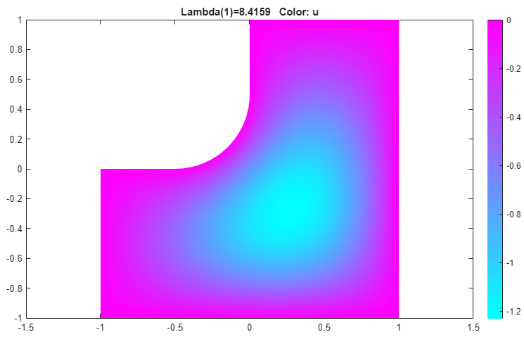
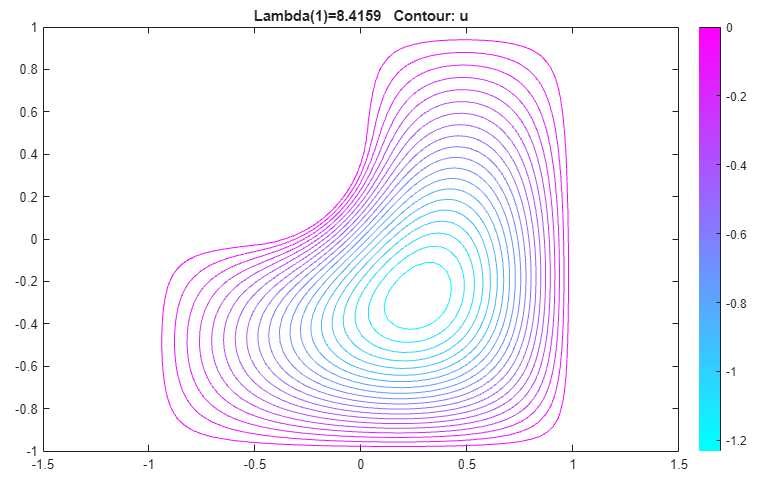
12. Plot the same eigenfunction as a contour plot. To do this:

    1. Select Plot > Parameters.

    2. Clear the Color option and select the Contour option.