線形計画法を使用した長期投資の運用最大化: ソルバーベース

ライブスクリプトを開く

この例では、Optimization Toolbox® の linprog ソルバーを使用して、固定の年数 T にわたって確定的なリターンがある投資の問題を解く方法を説明します。この問題は利用可能な投資に資金を割り当てて最終資産額を最大化するものです。この例では、ソルバーベースのアプローチを使用します。

問題の定式化

N 個のゼロクーポン債に T 年の期間にわたって投資するための初期資金 Capital_0 があるとします。各債券の支払い利率は年単位の複利で、満期時に元本と複利が支払われます。目的は T 年後の総資産額を最大化することです。

単一の投資が総資本の特定の割合を超えないようにする制約を含めることができます。

この例では、まず小規模なケースで問題の設定を示し、次に一般的なケースに定式化します。

この問題は、線形計画問題としてモデル化できます。そこで、資産額を最適化するような、linprog ソルバーによる求解問題を策定します。

基本的な例

まず、小規模な例から始めます。

初期投資額 Capital_0 は $1000 です。
期間 T は 5 年です。
債券数 N は 4 です。
未投資資金をモデル化するために、満期が 1 年、利率が 0% で毎年利用可能な 1 つのオプション B0 を設定します。
債券 1 は B1 で表され、1 年目に購入でき、満期は 4 年、利率は 2% です。
債券 2 は B2 で表され、5 年目に購入でき、満期は 1 年、利率は 4% です。
債券 3 は B3 で表され、2 年目に購入でき、満期は 4 年、利率は 6% です。
債券 4 は B4 で表され、2 年目に購入でき、満期は 3 年、利率は 6% です。

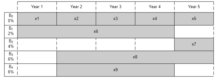
最初のオプション B0 を満期が 1 年で利率が 0% の 5 つの債券に分割することによって、利用可能な債券合計数が 9 であるとしてこの問題を等価的にモデル化できます。つまり、k=1..9 に対して、次のとおりとします。

ベクトル PurchaseYears のエントリ k は、債券 k を購入可能な年を表します。
ベクトル Maturity のエントリ k は、債券 k の満期 $m_{k}$ を表します。
ベクトル InterestRates のエントリ k は、債券 k の利率 $ρ_{k}$ を表します。

各債券の購入可能回数と期間を水平のバーで表すことによって、この問題を視覚化します。

% Time period in years
T = 5;
% Number of bonds
N = 4;
% Initial amount of money
Capital_0 = 1000;
% Total number of buying opportunities
nPtotal = N+T;
% Purchase times
PurchaseYears = [1;2;3;4;5;1;5;2;2];
% Bond durations
Maturity = [1;1;1;1;1;4;1;4;3];
% Interest rates
InterestRates = [0;0;0;0;0;2;4;6;6];

plotInvestments(N,PurchaseYears,Maturity,InterestRates)

決定変数

ベクトル x によって決定変数を表します。ここで、x(k) は、債券 k (k=1..9) へのドル建て投資額です。満期時の投資 x(k) に対する支払いは次のようになります。

$x (k) (1 + ρ_{k} / 100)^{m_{k}} .$

$β_{k} = 1 + ρ_{k} / 100$ を定義し、 $r_{k}$ を債券 k のトータルリターンとして定義します。

$r_{k} = (1 + ρ_{k} / 100)^{m_{k}} = β_{k}^{m_{k}} .$

% Total returns
finalReturns = (1+InterestRates/100).^Maturity;

目的関数

ゴールは T 年目の終わりに回収される金額を最大化する投資を選択することです。プロットから、投資は中間のさまざまな年に回収され、再投資されることがわかります。T 年目の終わりに投資 5、7、および 8 からリターンを回収でき、最終資産額は次のように表されます。

$\max_{x} x_{5} r_{5} + x_{7} r_{7} + x_{8} r_{8}$

この問題を linprog ソルバー形式にするには、符号反転した x(j) の係数を使用して、最大化問題から最小化問題に変換します。

$\min_{x} f^{T} x$

に対し

$f = [0; 0; 0; 0; - r_{5}; 0; - r_{7}; - r_{8}; 0]$

f = zeros(nPtotal,1);
f([5,7,8]) = [-finalReturns(5),-finalReturns(7),-finalReturns(8)];

線形制約: 保有金額を超えて投資しない

毎年、一定金額を債券の購入に利用できます。まず 1 年目には、初期資本を購入オプション $x_{1}$ および $x_{6}$ に投資できるため、次のようになります。

$x_{1} + x_{6} = {C a p i t a l}_{0}$

その後の年では、満期になった債券からリターンを回収し、利用可能な新しい債券に再投資するため、次の方程式系が得られます。

$\begin{array}{ll} x_{2} + x_{8} + x_{9} & = r_{1} x_{1} \\ x_{3} & = r_{2} x_{2} \\ x_{4} & = r_{3} x_{3} \\ x_{5} + x_{7} & = r_{4} x_{4} + r_{6} x_{6} + r_{9} x_{9} \end{array}$

これらの方程式を $A e q x = b e q$ の形式で記述します。ここで、 $A e q$ 行列の各行は、その年に満たす必要がある等式に相当します。

$A e q = [\begin{array}{ccccccccc} 1 & 0 & 0 & 0 & 0 & 1 & 0 & 0 & 0 \\ - r_{1} & 1 & 0 & 0 & 0 & 0 & 0 & 1 & 1 \\ 0 & - r_{2} & 1 & 0 & 0 & 0 & 0 & 0 & 0 \\ 0 & 0 & - r_{3} & 1 & 0 & 0 & 0 & 0 & 0 \\ 0 & 0 & 0 & - r_{4} & 1 & - r_{6} & 1 & 0 & - r_{9} \end{array}]$

$b e q = [\begin{array}{c} {C a p i t a l}_{0} \\ 0 \\ 0 \\ 0 \end{array}]$

Aeq = spalloc(N+1,nPtotal,15);
Aeq(1,[1,6]) = 1;
Aeq(2,[1,2,8,9]) = [-1,1,1,1];
Aeq(3,[2,3]) = [-1,1];
Aeq(4,[3,4]) = [-1,1];
Aeq(5,[4:7,9]) = [-finalReturns(4),1,-finalReturns(6),1,-finalReturns(9)];

beq = zeros(T,1);
beq(1) = Capital_0;

範囲制約: 借入をしない

各投資金額が正の値でなければならないため、解ベクトル $x$ の各エントリは正の値でなければなりません。解ベクトル $x$ に下限 lb を設定して、この制約を含めます。解ベクトルには明示的な上限はありません。つまり、上限 ub を空に設定します。

lb = zeros(size(f));
ub = [];

問題を解く

債券に投資できる金額に制約を付けずにこの問題を解きます。このような線形計画問題を解くには、内点法アルゴリズムを使用できます。

options = optimoptions('linprog','Algorithm','interior-point');
[xsol,fval,exitflag] = linprog(f,[],[],Aeq,beq,lb,ub,options);

Solution found during presolve.

解の可視化

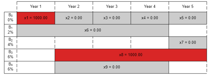
終了フラグは 1 で、ソルバーによって解が見つかったことを示しています。linprog の 2 番目の出力引数として返される値 -fval は、最終資産額に相当します。時間の経過に合わせて投資額をプロットします。

fprintf('After %d years, the return for the initial $%g is $%g \n',...
    T,Capital_0,-fval);

After 5 years, the return for the initial $1000 is $1262.48

plotInvestments(N,PurchaseYears,Maturity,InterestRates,xsol)

保有債券に制限がある場合の最適な投資

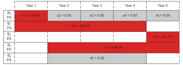
投資を分散するために、1 つの債券に投資する金額を、その年の総資本 (その時点で満期になっている債券のリターンを含む) の特定の割合 Pmax に制限するよう選択することもできます。次の連立不等式が得られます。

$\begin{array}{ll} x_{1} & \leq P m a x \times {C a p i t a l}_{0} \\ x_{2} & \leq P m a x \times (β_{1} x_{1} + β_{6} x_{6}) \\ x_{3} & \leq P m a x \times (β_{2} x_{2} + β_{6}^{2} x_{6} + β_{8} x_{8} + β_{9} x_{9}) \\ x_{4} & \leq P m a x \times (β_{3} x_{3} + β_{6}^{3} x_{6} + β_{8}^{2} x_{8} + β_{9}^{2} x_{9}) \\ x_{5} & \leq P m a x \times (β_{4} x_{4} + β_{6}^{4} x_{4} + β_{8}^{3} x_{8} + β_{9}^{3} x_{9}) \\ x_{6} & \leq P m a x \times {C a p i t a l}_{0} \\ x_{7} & \leq P m a x \times (β_{4} x_{4} + β_{6}^{4} x_{4} + β_{8}^{3} x_{8} + β_{9}^{3} x_{9}) \\ x_{8} & \leq P m a x \times (β_{1} x_{1} + β_{6} x_{6}) \\ x_{9} & \leq P m a x \times (β_{1} x_{1} + β_{6} x_{6}) \end{array}$

これらの不等式を行列の形式 Ax <= b にします。

連立不等式を設定するには、まず i 行目の j 列が j 年目の債券 i のリターンである行列 yearlyReturns を生成します。この連立不等式をスパース行列として表します。

% Maximum percentage to invest in any bond
Pmax = 0.6;

% Build the return for each bond over the maturity period as a sparse
% matrix
cumMaturity = [0;cumsum(Maturity)];
xr = zeros(cumMaturity(end-1),1);
yr = zeros(cumMaturity(end-1),1);
cr = zeros(cumMaturity(end-1),1);
for i = 1:nPtotal
    mi = Maturity(i); % maturity of bond i
    pi = PurchaseYears(i); % purchase year of bond i
    idx = cumMaturity(i)+1:cumMaturity(i+1); % index into xr, yr and cr
    xr(idx) = i; % bond index
    yr(idx) = pi+1:pi+mi; % maturing years
    cr(idx) = (1+InterestRates(i)/100).^(1:mi); % returns over the maturity period
end
yearlyReturns = sparse(xr,yr,cr,nPtotal,T+1);

% Build the system of inequality constraints
A = -Pmax*yearlyReturns(:,PurchaseYears)'+ speye(nPtotal);

% Left-hand side
b = zeros(nPtotal,1);
b(PurchaseYears == 1) = Pmax*Capital_0;

どの資産への投資も 60% を超えないようにして問題を解きます。結果として得られる購入額をプロットします。この制約なしに投資する場合より最終資産額が少なくなることがわかります。

[xsol,fval,exitflag] = linprog(f,A,b,Aeq,beq,lb,ub,options);

Minimum found that satisfies the constraints.

Optimization completed because the objective function is non-decreasing in feasible directions, to within the function tolerance, and constraints are satisfied to within the constraint tolerance.

fprintf('After %d years, the return for the initial $%g is $%g \n',...
    T,Capital_0,-fval);

After 5 years, the return for the initial $1000 is $1207.78

plotInvestments(N,PurchaseYears,Maturity,InterestRates,xsol)

任意のサイズのモデル

一般的な問題のモデルを作成します。T = 30 年、利率が 1 ～ 6% でランダムに生成された 400 個の債券を使用してこのモデルを説明します。この設定の場合、決定変数が 430 個ある線形計画問題になります。連立等式制約は、次元が 30 行 430 列のスパース行列 Aeq で表され、連立不等式制約は、次元が 430 行 430 列のスパース行列 A で表されます。

% for reproducibility
rng default 
% Initial amount of money
Capital_0 = 1000;
% Time period in years
T = 30;
% Number of bonds
N = 400;
% Total number of buying opportunities
nPtotal = N+T;
% Generate random maturity durations
Maturity = randi([1 T-1],nPtotal,1);
% Bond 1 has a maturity period of 1 year
Maturity(1:T) = 1;
% Generate random yearly interest rate for each bond
InterestRates = randi(6,nPtotal,1);
% Bond 1 has an interest rate of 0 (not invested)
InterestRates(1:T) = 0;
% Compute the return at the end of the maturity period for each bond:
finalReturns = (1+InterestRates/100).^Maturity;

% Generate random purchase years for each option
PurchaseYears = zeros(nPtotal,1);
% Bond 1 is available for purchase every year
PurchaseYears(1:T)=1:T;
for i=1:N
    % Generate a random year for the bond to mature before the end of
    % the T year period
    PurchaseYears(i+T) = randi([1 T-Maturity(i+T)+1]);
end

% Compute the years where each bond reaches maturity
SaleYears = PurchaseYears + Maturity;

% Initialize f to 0
f = zeros(nPtotal,1);
% Indices of the sale opportunities at the end of year T
SalesTidx = SaleYears==T+1;
% Expected return for the sale opportunities at the end of year T
ReturnsT = finalReturns(SalesTidx);
% Objective function
f(SalesTidx) = -ReturnsT;


% Generate the system of equality constraints.
% For each purchase option, put a coefficient of 1 in the row corresponding
% to the year for the purchase option and the column corresponding to the
% index of the purchase oportunity
xeq1 = PurchaseYears;
yeq1 = (1:nPtotal)';
ceq1 = ones(nPtotal,1);

% For each sale option, put -\rho_k, where \rho_k is the interest rate for the
% associated bond that is being sold, in the row corresponding to the
% year for the sale option and the column corresponding to the purchase
% oportunity
xeq2 = SaleYears(~SalesTidx);
yeq2 = find(~SalesTidx);
ceq2 = -finalReturns(~SalesTidx);

% Generate the sparse equality matrix
Aeq = sparse([xeq1; xeq2], [yeq1; yeq2], [ceq1; ceq2], T, nPtotal);

% Generate the right-hand side
beq = zeros(T,1);
beq(1) = Capital_0;

% Build the system of inequality constraints
% Maximum percentage to invest in any bond
Pmax = 0.4;

% Build the returns for each bond over the maturity period
cumMaturity = [0;cumsum(Maturity)];
xr = zeros(cumMaturity(end-1),1);
yr = zeros(cumMaturity(end-1),1);
cr = zeros(cumMaturity(end-1),1);
for i = 1:nPtotal
    mi = Maturity(i); % maturity of bond i
    pi = PurchaseYears(i); % purchase year of bond i
    idx = cumMaturity(i)+1:cumMaturity(i+1); % index into xr, yr and cr
    xr(idx) = i; % bond index
    yr(idx) = pi+1:pi+mi; % maturing years
    cr(idx) = (1+InterestRates(i)/100).^(1:mi); % returns over the maturity period
end
yearlyReturns = sparse(xr,yr,cr,nPtotal,T+1);

% Build the system of inequality constraints
A = -Pmax*yearlyReturns(:,PurchaseYears)'+ speye(nPtotal);

% Left-hand side
b = zeros(nPtotal,1);
b(PurchaseYears==1) = Pmax*Capital_0;

% Add the lower-bound constraints to the problem.
lb = zeros(nPtotal,1);

保有債券に制限がない場合の解

まず、内点法アルゴリズムを使用して不等式制約のない線形計画問題を解きます。

% Solve the problem without inequality constraints
options = optimoptions('linprog','Algorithm','interior-point');
tic
[xsol,fval,exitflag] = linprog(f,[],[],Aeq,beq,lb,[],options);

Minimum found that satisfies the constraints.

Optimization completed because the objective function is non-decreasing in feasible directions, to within the function tolerance, and constraints are satisfied to within the constraint tolerance.

toc

Elapsed time is 0.029424 seconds.

fprintf('\nAfter %d years, the return for the initial $%g is $%g \n',...
    T,Capital_0,-fval);

After 30 years, the return for the initial $1000 is $5167.58

保有債券に制限がある場合の解

次に、不等式制約のある問題を解きます。

% Solve the problem with inequality constraints
options = optimoptions('linprog','Algorithm','interior-point');
tic
[xsol,fval,exitflag] = linprog(f,A,b,Aeq,beq,lb,[],options);

Minimum found that satisfies the constraints.

Optimization completed because the objective function is non-decreasing in feasible directions, to within the function tolerance, and constraints are satisfied to within the constraint tolerance.

toc

Elapsed time is 0.706665 seconds.

fprintf('\nAfter %d years, the return for the initial $%g is $%g \n',...
    T,Capital_0,-fval);

After 30 years, the return for the initial $1000 is $5095.26

制約の数は 10 のオーダーで増加するのに対して、ソルバーによって解が見つけられるまでの時間は 100 のオーダーで増加します。このようなパフォーマンスの不一致が生じる原因の 1 つは、行列 A で示す連立不等式に密な列が含まれるためです。次のグラフからわかるように、これらの列は長期満期の債券に相当します。

% Number of nonzero elements per column
nnzCol = sum(spones(A));

% Plot the maturity length vs. the number of nonzero elements for each bond
figure;
plot(Maturity,nnzCol,'o');
xlabel('Maturity period of bond k')
ylabel('Number of nonzero in column k of A')

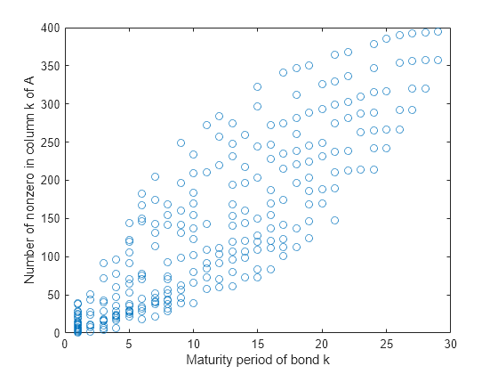
制約内の密な列によってソルバーの内部行列に密なブロックが生じ、スパース法の効率が損なわれます。ソルバーのスピードを向上させるため、列密度の影響をあまり受けない双対シンプレックス法アルゴリズムを使用してみます。

% Solve the problem with inequality constraints using dual simplex
options = optimoptions('linprog','Algorithm','dual-simplex');
tic
[xsol,fval,exitflag] = linprog(f,A,b,Aeq,beq,lb,[],options);

Optimal solution found.

toc

Elapsed time is 0.080887 seconds.

fprintf('\nAfter %d years, the return for the initial $%g is $%g \n',...
    T,Capital_0,-fval);

After 30 years, the return for the initial $1000 is $5095.26

このケースでは、双対シンプレックス法アルゴリズムは同じ解を得るまでの時間を大幅に短縮しました。

定性結果分析

linprog によって見つかった解の特性を確認するため、この解を、初期資金の全額を利率 6% (最大利率) の 1 つの債券に 30 年間にわたって投資した場合に得られる金額 fmax と比較します。最終資産額に対応する同等の利率を計算することもできます。

% Maximum amount
fmax = Capital_0*(1+6/100)^T;
% Ratio (in percent)
rat = -fval/fmax*100;
% Equivalent interest rate (in percent)
rsol = ((-fval/Capital_0)^(1/T)-1)*100;

fprintf(['The amount collected is %g%% of the maximum amount $%g '...
    'that you would obtain from investing in one bond.\n'...
    'Your final wealth corresponds to a %g%% interest rate over the %d year '...
    'period.\n'], rat, fmax, rsol, T)

The amount collected is 88.7137% of the maximum amount $5743.49 that you would obtain from investing in one bond.
Your final wealth corresponds to a 5.57771% interest rate over the 30 year period.

plotInvestments(N,PurchaseYears,Maturity,InterestRates,xsol,false)