工場、倉庫、販売店割り当てモデル: ソルバーベース

ライブスクリプトを開く

この例では、混合整数線形計画問題を設定および解決する方法を説明します。問題は、一連の工場、倉庫、販売店間の生産および流通の最適レベルを求めることです。問題ベースのアプローチについては、工場、倉庫、販売店割り当てモデル: 問題ベースを参照してください。

この例では、まず工場、倉庫、販売店のランダムな位置を生成します。スケーリングパラメーター $N$ を自由に変更して、生産および流通施設が配置されている両方のグリッドのサイズをスケーリングすると共に、グリッドエリアの各タイプの施設の密度が $N$ に依存しないように、これらの施設の数をスケーリングします。

施設の位置

特定のスケーリングパラメーターの値 $N$ には以下があるとします。

$⌊ f N^{2} ⌋$ 個の工場
$⌊ w N^{2} ⌋$ 個の倉庫
$⌊ s N^{2} ⌋$ 個の販売店

これらの施設は、 $x$ および $y$ 方向で 1 と $N$ の間にある別個の整数グリッド点にあります。施設が別個の位置をもつためには、 $f + w + s \leq 1$ である必要があります。この例では、 $N = 20$ 、 $f = 0.05$ 、 $w = 0.05$ 、 $s = 0.1$ とします。

生産および流通

工場では、 $P$ 個の製品が製造されています。 $P = 20$ とします。

販売店 $s$ における各製品 $p$ の需要は $d (s, p)$ です。需要とは、ある期間において販売可能な数量です。このモデルの制約の 1 つは需要を満たすことです。つまり、システムが需要に厳密に見合う数量を生産および供給することです。

各工場および倉庫には能力の制約があります。

工場 $f$ における製品 $p$ の生産は $p c a p (f, p)$ 未満です。
倉庫 $w$ の容量は $w c a p (w)$ です。
特定の期間に倉庫 $w$ から販売店に輸送できる製品 $p$ の数量は $t u r n (p) * w c a p (w)$ 未満です。ここで、 $t u r n (p)$ は製品 $p$ の回転率です。

各販売店は 1 つの倉庫からのみ供給を受けるものとします。問題の一部として、倉庫に対し販売店を最も低コストに配置することがあります。

コスト

工場から倉庫および倉庫から販売店までの製品輸送コストは、施設間の距離および製品ごとに異なります。 $d i s t (a, b)$ が施設 $a$ と $b$ の間の距離であるとすると、これらの施設間で製品 $p$ を出荷するコストは輸送コスト $t c o s t (p)$ に距離を乗算した値になります。

$d i s t (a, b) * t c o s t (p) .$

この例における距離は $L_{1}$ 距離とも呼ばれるグリッド距離です。これは $x$ 座標と $y$ 座標の差の絶対値の総和です。

工場 $f$ で製品 $p$ を 1 単位生産するコストは $p c o s t (f, p)$ です。

最適化問題

一連の施設の位置と需要および能力の制約を所与として、以下を求めます。

各工場における各製品の生産レベル
工場から倉庫への製品の出荷スケジュール
倉庫から販売店への製品の出荷スケジュール

これらの数量は、需要が満たされ、総コストが最小化されるものでなければなりません。また、各販売店はすべての製品を 1 つの倉庫からのみ受け取る必要があります。

最適化問題の変数と方程式

制御変数 (最適化において変更可能な変数) は以下のとおりです。

$x (p, f, w)$ = 工場 $f$ から倉庫 $w$ に輸送する製品 $p$ の数量
$y (s, w)$ = 販売店 $s$ が倉庫 $w$ と関連付けられているときに値が 1 になるバイナリ変数

最小化する目的関数は以下のとおりです。

$\sum_{f} \sum_{p} \sum_{w} x (p, f, w) \cdot (p c o s t (f, p) + t c o s t (p) \cdot d i s t (f, w))$

$+ \sum_{s} \sum_{w} \sum_{p} (d (s, p) \cdot t c o s t (p) \cdot d i s t (s, w) \cdot y (s, w)) .$

制約は次のとおりです。

$\sum_{w} x (p, f, w) \leq p c a p (f, p)$ (工場の能力)。

$\sum_{f} x (p, f, w) = \sum_{s} (d (s, p) \cdot y (s, w))$ (需要を満たす)。

$\sum_{p} \sum_{s} \frac{d (s, p)}{t u r n (p)} \cdot y (s, w) \leq w c a p (w)$ (倉庫の容量)。

$\sum_{w} y (s, w) = 1$ (各販売店が 1 つの倉庫に関連付けられている)。

$x (p, f, w) \geq 0$ (非負の生産)。

$y (s, w) ϵ {0, 1}$ (バイナリの $y$ )。

変数 $x$ および $y$ は、目的関数と制約関数で線形になります。 $y$ は整数値に制限されるため、問題は混合整数線形計画法 (MILP) になります。

ランダムな問題の生成: 施設の位置

パラメーター $N$ 、 $f$ 、 $w$ および $s$ の値を設定し、施設の位置を生成します。

rng(1) % for reproducibility
N = 20; % N from 10 to 30 seems to work. Choose large values with caution.
N2 = N*N;
f = 0.05; % density of factories
w = 0.05; % density of warehouses
s = 0.1; % density of sales outlets

F = floor(f*N2); % number of factories
W = floor(w*N2); % number of warehouses
S = floor(s*N2); % number of sales outlets

xyloc = randperm(N2,F+W+S); % unique locations of facilities
[xloc,yloc] = ind2sub([N N],xyloc);

もちろん、施設の位置を無作為に指定するのは現実的ではありません。この例は、解決法を示すことを目的としたものであり、適切な施設の位置を生成する方法を示すものではありません。

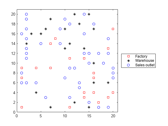
施設をプロットします。施設 1 ～ F は工場、F+1 ～ F+W は倉庫、F+W+1 ～ F+W+S は販売店です。

h = figure;
plot(xloc(1:F),yloc(1:F),'rs',xloc(F+1:F+W),yloc(F+1:F+W),'k*',...
    xloc(F+W+1:F+W+S),yloc(F+W+1:F+W+S),'bo');
lgnd = legend('Factory','Warehouse','Sales outlet','Location','EastOutside');
lgnd.AutoUpdate = 'off';
xlim([0 N+1]);ylim([0 N+1])

Figure contains an axes object. The axes object contains 3 objects of type line. One or more of the lines displays its values using only markers These objects represent Factory, Warehouse, Sales outlet.

ランダムな能力、コストおよび需要の生成

ランダムな生産コスト、能力、回転率および需要を生成します。

P = 20; % 20 products

% Production costs between 20 and 100
pcost = 80*rand(F,P) + 20;

% Production capacity between 500 and 1500 for each product/factory
pcap = 1000*rand(F,P) + 500;

% Warehouse capacity between P*400 and P*800 for each product/warehouse
wcap = P*400*rand(W,1) + P*400;

% Product turnover rate between 1 and 3 for each product
turn = 2*rand(1,P) + 1;

% Product transport cost per distance between 5 and 10 for each product
tcost = 5*rand(1,P) + 5;

% Product demand by sales outlet between 200 and 500 for each
% product/outlet
d = 300*rand(S,P) + 200;

これらのランダムな需要と能力によって実行不可能な問題につながることがあります。つまり、需要が生産と倉庫の能力を超える場合があります。パラメーターを変更して実行不可能な問題が発生した場合、解を生成する際に終了フラグ -2 が表示されます。

目的関数および制約の行列とベクトルの生成

intlincon の目的関数ベクトル obj は、変数 $x (p, f, w)$ および $y (s, w)$ の係数で構成されます。したがって、当然 obj には P*F*W + S*W 係数が存在します。

係数を生成する 1 つの方法は、 $x$ 係数に P-by-F-by-W 配列 obj1、 $y (s, w)$ 係数に S-by-W 配列 obj2 を使用して開始することです。次にこれらの配列を 2 つのベクトルに変換し、以下を呼び出すことによって、これらを obj に結合します。

obj = [obj1(:);obj2(:)];

obj1 = zeros(P,F,W); % Allocate arrays
obj2 = zeros(S,W);

目的関数および制約のベクトルと行列の生成全体を通じて、 $(p, f, w)$ 配列または $(s, w)$ 配列を生成し、その結果をベクトルに変換します。

入力の生成を開始するには、距離の配列 distfw(i,j) と distsw(i,j) を生成します。

distfw = zeros(F,W); % Allocate matrix for factory-warehouse distances
for ii = 1:F
    for jj = 1:W
        distfw(ii,jj) = abs(xloc(ii) - xloc(F + jj)) + abs(yloc(ii) ...
            - yloc(F + jj));
    end
end

distsw = zeros(S,W); % Allocate matrix for sales outlet-warehouse distances
for ii = 1:S
    for jj = 1:W
        distsw(ii,jj) = abs(xloc(F + W + ii) - xloc(F + jj)) ...
            + abs(yloc(F + W + ii) - yloc(F + jj));
    end
end

obj1 と obj2 のエントリを生成します。

for ii = 1:P
    for jj = 1:F
        for kk = 1:W
            obj1(ii,jj,kk) = pcost(jj,ii) + tcost(ii)*distfw(jj,kk);
        end
    end
end

for ii = 1:S
    for jj = 1:W
        obj2(ii,jj) = distsw(ii,jj)*sum(d(ii,:).*tcost);
    end
end

エントリを 1 つのベクトルに結合します。

obj = [obj1(:);obj2(:)]; % obj is the objective function vector

ここで制約行列を作成します。

各線形制約行列の幅は obj ベクトルの長さです。

matwid = length(obj);

線形不等式には、生産能力の制約と倉庫能力の制約の 2 種類があります。

生産能力の制約 P*F と倉庫能力の制約 W があります。制約行列は 1% 非ゼロの順序できわめて疎であるため、スパース行列を使ってメモリを保存します。

Aineq = spalloc(P*F + W,matwid,P*F*W + S*W); % Allocate sparse Aeq
bineq = zeros(P*F + W,1); % Allocate bineq as full

% Zero matrices of convenient sizes:
clearer1 = zeros(size(obj1));
clearer12 = clearer1(:);
clearer2 = zeros(size(obj2));
clearer22 = clearer2(:);

% First the production capacity constraints
counter = 1;
for ii = 1:F
    for jj = 1:P
        xtemp = clearer1;
        xtemp(jj,ii,:) = 1; % Sum over warehouses for each product and factory
        xtemp = sparse([xtemp(:);clearer22]); % Convert to sparse
        Aineq(counter,:) = xtemp'; % Fill in the row
        bineq(counter) = pcap(ii,jj);
        counter = counter + 1;
    end
end

% Now the warehouse capacity constraints
vj = zeros(S,1); % The multipliers 
for jj = 1:S
    vj(jj) = sum(d(jj,:)./turn); % A sum of P elements
end

for ii = 1:W
    xtemp = clearer2;
    xtemp(:,ii) = vj;
    xtemp = sparse([clearer12;xtemp(:)]); % Convert to sparse
    Aineq(counter,:) = xtemp'; % Fill in the row
    bineq(counter) = wcap(ii);
    counter = counter + 1;
end

線形等式制約には、需要を満たす制約と各販売店が 1 つの倉庫に対応する制約の 2 種類があります。

Aeq = spalloc(P*W + S,matwid,P*W*(F+S) + S*W); % Allocate as sparse
beq = zeros(P*W + S,1); % Allocate vectors as full

counter = 1;
% Demand is satisfied:
for ii = 1:P
    for jj = 1:W
        xtemp = clearer1;
        xtemp(ii,:,jj) = 1;
        xtemp2 = clearer2;
        xtemp2(:,jj) = -d(:,ii);
        xtemp = sparse([xtemp(:);xtemp2(:)]'); % Change to sparse row
        Aeq(counter,:) = xtemp; % Fill in row
        counter = counter + 1;
    end
end

% Only one warehouse for each sales outlet:
for ii = 1:S
    xtemp = clearer2;
    xtemp(ii,:) = 1;
    xtemp = sparse([clearer12;xtemp(:)]'); % Change to sparse row
    Aeq(counter,:) = xtemp; % Fill in row
    beq(counter) = 1;
    counter = counter + 1;
end

範囲制約と整数変数

整数変数は length(obj1) + 1 から最後までとなります。

intcon = P*F*W+1:length(obj);

上限も length(obj1) + 1 から最後までとなります。

lb = zeros(length(obj),1);
ub = Inf(length(obj),1);
ub(P*F*W+1:end) = 1;

何百もの出力の線が表示されないように、反復表示をオフにします。解決進行状況を監視するためのプロット関数を含めます。

opts = optimoptions('intlinprog','Display','off','PlotFcn',@optimplotmilp);

問題を解く

ソルバーの入力がすべて生成されました。ソルバーを呼び出して解を求めます。

[solution,fval,exitflag,output] = intlinprog(obj,intcon,...
                                     Aineq,bineq,Aeq,beq,lb,ub,opts);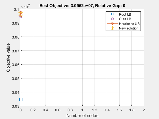

Figure Optimization Plot Function contains an axes object. The axes object with title Best Objective: 3.0952e+07, Relative Gap: 0, xlabel Number of nodes, ylabel Objective value contains 4 objects of type line. One or more of the lines displays its values using only markers These objects represent Root LB, Cuts LB, Heuristics UB, New solution.

if isempty(solution) % If the problem is infeasible or you stopped early with no solution
    disp('intlinprog did not return a solution.')
    return % Stop the script because there is nothing to examine
end

解の検証

解は指定された許容誤差の範囲内で実行可能です。

exitflag

exitflag = 1

infeas1 = max(Aineq*solution - bineq)

infeas1 = 2.5011e-12

infeas2 = norm(Aeq*solution - beq,Inf)

infeas2 = 1.7621e-12

整数要素が確かに整数であるかまたは丸めて十分整数に近い妥当な値になるかを確認します。これらの変数が厳密に整数ではない可能性がある理由を理解するには、一部の “整数” 解は整数ではないを参照してください。

diffint = norm(solution(intcon) - round(solution(intcon)),Inf)

diffint = 1.4433e-15

整数変数が厳密に整数ではない場合がありますが、すべて整数に非常に近い変数です。したがって整数変数を丸めます。

solution(intcon) = round(solution(intcon));

丸めた解の実行可能性と目的関数値の変更を確認します。

infeas1 = max(Aineq*solution - bineq)

infeas1 = 2.5011e-12

infeas2 = norm(Aeq*solution - beq,Inf)

infeas2 = 1.7621e-12

diffrounding = norm(fval - obj(:)'*solution,Inf)

diffrounding = 2.2352e-08

解の丸めによって、その実行可能性は目につくほどには変更されませんでした。

解を検証する最も簡単な方法は、解を変形して元の次元に戻すことです。

solution1 = solution(1:P*F*W); % The continuous variables
solution2 = solution(intcon); % The integer variables
solution1 = reshape(solution1,P,F,W);
solution2 = reshape(solution2,S,W);

たとえば、各倉庫に関連付けられている販売店数はいくつでしょうか。この場合、一部の倉庫は関連付けられた店舗がゼロであることに注意してください。これは、倉庫が最適解で使用されていないことを示します。

outlets = sum(solution2,1) % Sum over the sales outlets

outlets = 1×20

     3     0     3     2     2     2     3     2     3     1     1     0     0     3     4     3     2     3     2     1

各販売店とその倉庫間の接続をプロットします。

figure(h);
hold on
for ii = 1:S
    jj = find(solution2(ii,:)); % Index of warehouse associated with ii
    xsales = xloc(F+W+ii); ysales = yloc(F+W+ii);
    xwarehouse = xloc(F+jj); ywarehouse = yloc(F+jj);
    if rand(1) < .5 % Draw y direction first half the time
        plot([xsales,xsales,xwarehouse],[ysales,ywarehouse,ywarehouse],'g--')
    else % Draw x direction first the rest of the time
        plot([xsales,xwarehouse,xwarehouse],[ysales,ysales,ywarehouse],'g--')
    end
end
hold off

title('Mapping of sales outlets to warehouses')

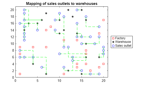
Figure contains an axes object. The axes object with title Mapping of sales outlets to warehouses contains 43 objects of type line. One or more of the lines displays its values using only markers These objects represent Factory, Warehouse, Sales outlet.

緑色の線がない黒い * は使用されない倉庫を表します。