Optimize Pressure Reducing Valve Model for Real-Time Simulation

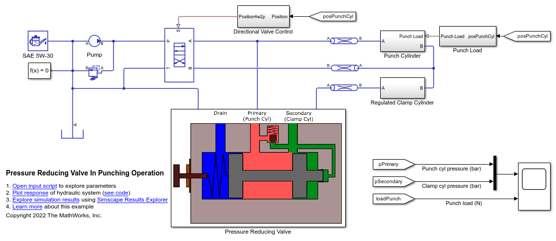
This example shows how to identify simulation slowdowns, resolve performance issues, and configure a Simscape Fluids™ model for real-time simulation. This example uses the Pressure Reducing Valve In Punching Operation model, PressureReducingValveInPunchingOperation which is called here as the original model. In this example, you measure the simulation time, identify the factors that affect simulation speed, optimize the model, and prepare the model for code generation.

Open and Examine the Model

Open the original model.

model = 'PressureReducingValveInPunchingOperation';
open_system(model)

The model has been configured for real-time simulation by performing these steps:

1. Enable the Use local solver option in the Solver Configuration block. Set Solver type to Backward Euler and Sample time to 2e-4. Enable the Use fixed-cost runtime consistency iterations option in the Solver Configuration block. Expand the Use fixed-cost runtime consistency iterations option and set Nonlinear iterations to 3.

2. Open the Configuration Parameters window, click Solver, under Solver selection, set Type to Fixed-step, set Solver to ode1be (Backward Euler), and under Solver details, set Fixed-step size to 2e-4.

3. Replace Single-Acting Actuator (IL) blocks with Foundation Library blocks such as the Translational Mechanical Converter (IL), Translational Spring, Translational Damper and Translational Hard Stop blocks. Set Hard stop model in Translational Hard Stop block to Full stiffness and damping applied at bounds, damped rebound.

4. Convert the Punch Load and Directional Valve Control subsystems to Atomic Subsystems. Right click on the subsystems, then click Block Parameters (subsystem). Enable the Treat as atomic unit option and set the Sample time to 1e-3. Add Rate Transition blocks at the input and output of the subsystems.

5. Set the Smoothing factor parameter of the 4-Way 2-Position Directional Valve and the Check Valve blocks to 0.1.

6. Remove the Pipe (IL), Pipe (IL)1 and Pipe (IL)2 blocks. To compensate for the pipe volume, increase the dead volume of the single-acting actuators that represent the punch cylinder, clamp cylinder and pressure reducing valve spool. Navigate inside Punch Cylinder subsystem. Increase the value of Dead volume in chamber A and Dead volume in chamber B parameters of the Punch Cylinder block from 1e-6 m^3 to 1e-3 m^3. Navigate inside Regulated Clamp Cylinder subsystem. Increase the value of Dead volume in chamber A and Dead volume in chamber B parameters of the Clamp Cylinder block from 1e-6 m^3 to 1e-3 m^3. Navigate inside Pressure Reducing Valve subsystem. Increase the value of Dead volume parameter of the Single-Acting Actuator (IL) and Single-Acting Actuator (IL)1 blocks from 1e-5 m^3 to 1e-4 m^3.

Open the real-time model.

modelRT = 'PressureReducingValveInRealTime';
open_system(modelRT)

Now, again open and examine the PressureReducingValveInPunchingOperation model.

open_system(model)

This model includes interactions between Simscape™, Simulink® and Stateflow®. The Simscape blocks represent the physical model of the pressure-reducing valve and the punch system. The Simulink blocks are used to measure and transmit signals across the model. Stateflow models the conditional actuation of a punch cylinder that involves a feedback loop. The model includes several Goto, From, and PMC Port blocks that the subsystems use to interact with each other. This complex communication across the model causes simulation slowdown.

The Switch, Saturation, Hard Stop, Translational Friction blocks cause non-linear behavior that causes the solver to iterate using lower time steps. The 4-Way 2-Position Directional Valve causes changes in the flow direction which causes zero-crossings when the punch cylinder starts to displace or comes to a stop. The clamp cylinder and the pressure reducing valve spool cause similar behavior when they start to displace or come to a stop. These zero-crossings contribute to simulation slowdown.

The compressibility of the fluid is an essential aspect of modeling a hydraulic system. When the Fluid dynamic compressibility parameter of the Pipe block is set to On, an imbalance of mass inflow and mass outflow can cause liquid to accumulate or diminish in the pipe. As a result, pressure in the pipe volume can rise and fall dynamically, which provides some compliance to the system and modulates rapid pressure changes. This setting can contribute to simulation slowdown.

All the above factors can thus impede a real-time simulation. To achieve real-time simulation, the run time or execution time must be less than the Simulation stop time. To achieve real-time simulation for this model, you must use a fixed-step solver with a large enough time step.

Use a Variable-Step Solver to Get Reference Results

A variable-step solver adjusts the step size to capture events and dynamics in the system. Since, the variable step sizes cannot be mapped to the real-time clock of a target system, you must use an implicit or explicit fixed-step solver for real-time simulation.

To ensure that the results obtained with the fixed-step solver are accurate, compare them with reference results obtained by simulating the system with a variable-step solver.

To run your model using a variable-step solver, ensure that the Use local solver in the Solver Configuration block is set to off. This example focuses on reducing the elapsed simulation time for one cycle of punching operation. Set Simulation stop time (sec) to 6.

solverConfiguration = string(find_system(bdroot,'MaskType','Solver Configuration'));
set_param(solverConfiguration, 'UseLocalSolver', 'off');
set_param(model,'StopTime','6');

Before running the model, open the Configuration Parameters window, click Data Import/Export, then enable the Time parameter under Save to workspace or file tab. Enable the Single simulation output parameter to return simulation data as a single Simulink.SimulationOutput object. The object name is specified as out by default. Alternatively, enable the parameter by entering:

set_param(model,'SaveTime','on');
set_param(model,'ReturnWorkspaceOutputs','on');

Create a Simulink.SimulationInput object with Simulation stop time (sec) as an input argument.

simIn = Simulink.SimulationInput(model);
simIn = setModelParameter(simIn,'StopTime','6');

Specify a Simulink.SimulationOutput object. Run the model.

out = sim(simIn);

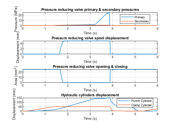
Plot the results.

figure;
PressureReducingValveInRealTimePlotVariableSolverResponse;

Examine Step Sizes during the Simulation

A variable-step solver will vary the step size to stay within the error tolerances and to react to zero-crossing events. If the solver abruptly reduces the step size to a small value (e.g., 1e-15s), this indicates that the solver is trying to accurately identify a zero-crossing event. A fixed-step solver may have trouble capturing these events at a step size large enough to permit real-time simulation. These MATLAB® commands can be used to generate a plot that shows how the time step varies during the simulation:

figure;
semilogy(out.tout(1:end-1),diff(out.tout),'-*');
title('Step Size vs. Simulation Time','FontSize',14,'FontWeight','bold');
xlabel('Simulation Time (s)','FontSize',12);
ylabel('Step Size (s)','FontSize',12);

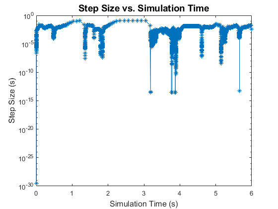
This plot shows the step sizes the solver takes during simulation. The sharp plunge in step size are examples of zero-crossing events.

This analysis should provide a rough idea of a step size that can be used to run the simulation. Determining what effects are causing these events and modifying or eliminating them will make it easier to run the system with a fixed-step solver at a larger step size and produce results comparable to the variable-step simulation.

A stiff system has continuous dynamics that vary slowly and quickly. Implicit solvers are particularly useful for stiff problems. Using an explicit solver to solve a stiff system can lead to incorrect results. If a nonstiff solver uses a very small step size to solve a model, this is a sign that your system is stiff. This plot shows that the variable-step solver takes very less step sizes and thus the system is stiff.

Use a Fixed-Step Solver to Measure Simulation Time

Run your model using fixed-step, fixed-cost configurations. It is recommended to enable the Use local solver option in the Solver Configuration block. Local solvers discretize the continuous states. Using local solvers permits configuring implicit solvers on the stiff portions of the model and explicit solvers on the remainder of the model, minimizing execution time while maintaining accuracy. This example uses the Backward Euler solver. Set Solver type to Backward Euler and Sample time to 1e-4. Enable the Use fixed-cost runtime consistency iterations option in the Solver Configuration block. Expand the Use fixed-cost runtime consistency iterations option and set Nonlinear iterations to 3.

set_param(solverConfiguration,'UseLocalSolver','on');
set_param(solverConfiguration,'LocalSolverChoice','NE_BACKWARD_EULER_ADVANCER');
set_param(solverConfiguration,'LocalSolverSampleTime','1e-4');
set_param(solverConfiguration,'LocalSolverSampleTime','1e-4');
set_param(solverConfiguration,'DoFixedCost','on');
set_param(solverConfiguration,'MaxNonlinIter','3');

Run the model.

simIn = Simulink.SimulationInput(model);
simIn = setModelParameter(simIn,'StopTime','6');
outBE1 = sim(simIn);

View the metadata and the timing information.

simMetadata = getSimulationMetadata(outBE1);
simMetadata.TimingInfo;

To see the elapsed simulation time, in seconds, enter:

simMetadata.TimingInfo.ExecutionElapsedWallTime;

The simulation time depends on the CPU on which you execute the model. There may be a difference between the time measured by you and the time in this example.

Compare Solvers and Determine if the Simulation runs Real-Time

Next, determine the fixed-step solver most appropriate for your model. To do this, use the local solvers in the Solver Configuration block and compare the elapsed simulation time for each. The available solvers are:

• Backward Euler

• Trapezoidal Rule

• Partitioning

The Backward Euler tends to damp out oscillations, but is more stable, especially if you increase the time step.

The Trapezoidal Rule solver captures oscillations better but is less stable.

The Partitioning solver lets you increase real-time simulation speed by partitioning the entire system of equations that correspond to a Simscape network into a cascade of smaller equation systems. Not all networks can be partitioned. However, when a system can be partitioned, this solver provides a significant increase in real-time simulation speed. To configure the Partitioning solver, set Solver type to Partitioning and Sample time to 1e-4. Set Partition method to Robust simulation and Partition storage method to Exhaustive. Enable the Use fixed-cost runtime consistency iterations option in the Solver Configuration block. Expand the Use fixed-cost runtime consistency iterations option and set Nonlinear iterations to 3.

set_param(solverConfiguration,'LocalSolverChoice','NE_PARTITIONING_ADVANCER');
set_param(solverConfiguration,'LocalSolverSampleTime','1e-4');
set_param(solverConfiguration,'PartitionMethod','ROBUST');
set_param(solverConfiguration,'PartitionStorageMethod','EXHAUSTIVE');
set_param(solverConfiguration,'DoFixedCost','on');
set_param(solverConfiguration,'MaxNonlinIter','3');

This system cannot be partitioned with a time step of 1e-4 s or greater.

Next, set Solver type to Backward Euler and Sample time to 1e-4. Enable the Use fixed-cost runtime consistency iterations option in the Solver Configuration block. Expand the Use fixed-cost runtime consistency iterations option and set Nonlinear iterations to 3.

set_param(solverConfiguration,'LocalSolverChoice','NE_BACKWARD_EULER_ADVANCER');
set_param(solverConfiguration,'LocalSolverSampleTime','1e-4');
set_param(solverConfiguration,'DoFixedCost','on');
set_param(solverConfiguration,'MaxNonlinIter','3');

Run the model.

simIn = Simulink.SimulationInput(model);
simIn = setModelParameter(simIn,'StopTime','6');
outBE1 = sim(simIn);

After running the model, access the metadata and the timing information.

simMetadata = getSimulationMetadata(outBE1);
simMetadata.TimingInfo;

View the elapsed simulation time, in seconds:

simMetadata.TimingInfo.ExecutionElapsedWallTime;

Then, set Solver type to Trapezoidal Rule and Sample time to 1e-4. Retain the fixed-cost configurations.

set_param(solverConfiguration,'LocalSolverChoice','NE_TRAPEZOIDAL_ADVANCER');
set_param(solverConfiguration,'LocalSolverSampleTime','1e-4');
set_param(solverConfiguration,'DoFixedCost','on');
set_param(solverConfiguration,'MaxNonlinIter','3');

Run the model.

simIn = Simulink.SimulationInput(model);
simIn = setModelParameter(simIn,'StopTime','6');
outTR1 = sim(simIn);

After running the model, access the metadata and the timing information.

simMetadata = getSimulationMetadata(outTR1);
simMetadata.TimingInfo;

View the elapsed simulation time, in seconds:

simMetadata.TimingInfo.ExecutionElapsedWallTime;

Because the elapsed simulation time is more than the Simulation stop time, the model does not run in real-time.

Identify Factors that Affect Speed and Choose an Appropriate Solution

Because the simulation is not real-time capable, you can explore some options.

• Determine New Settings that Reduce the Execution Time

You can either permit a larger step size or reduce the number of nonlinear iterations.

Again, set Solver type to Backward Euler. Now, set Sample time to 2e-4. Enable the Use fixed-cost runtime consistency iterations option in the Solver Configuration block. Expand the Use fixed-cost runtime consistency iterations option and set Nonlinear iterations to 3.

set_param(solverConfiguration,'LocalSolverChoice','NE_BACKWARD_EULER_ADVANCER');
set_param(solverConfiguration,'LocalSolverSampleTime','2e-4');
set_param(solverConfiguration,'DoFixedCost','on');
set_param(solverConfiguration,'MaxNonlinIter','3');

The global solver solves for the Simulink and Stateflow blocks. To ensure that the Simulink and Stateflow blocks also run at higher time steps without affecting accuracy, open the Configuration Parameters window, click Solver, under Solver selection, set Type to Fixed-step, set Solver to ode1be (Backward Euler), and under Solver details, set Fixed-step size to 2e-4.

set_param(model,'SolverType','Fixed-step');
set_param(model,'SolverName','ode1be');
set_param(model,'FixedStep','2e-4');

Run the model.

simIn = Simulink.SimulationInput(model);
simIn = setModelParameter(simIn,'StopTime','6');
outBE2 = sim(simIn);

Then, set Solver type to Trapezoidal Rule and Sample time to 2e-4. Retain the fixed-cost configurations.

set_param(solverConfiguration,'LocalSolverChoice','NE_TRAPEZOIDAL_ADVANCER');
set_param(solverConfiguration,'LocalSolverSampleTime','2e-4');
set_param(solverConfiguration,'DoFixedCost','on');
set_param(solverConfiguration,'MaxNonlinIter','3');

Run the model.

simIn = Simulink.SimulationInput(model);
simIn = setModelParameter(simIn,'StopTime','6');
outTR2 = sim(simIn);

Now, compare the results of simulation with large step size with the reference results obtained from variable-step solver.

figure;
PressureReducingValveInRealTimePlotSolverComparison;

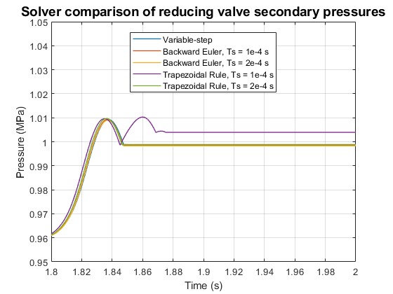
This zoomed in version of the figure shows the comparison of solvers for secondary pressure. Increasing the step size, increases the error, but the error is within acceptable limits for Backward Euler solver with sample time of 2e-4 s.

• Use the Solver Profiler to Identify Factors that Affect Speed

The system stiffness is high. High stiffness is responsible for simulation slowdown.

The Simscape Stiffness option in the Solver Profiler tool lets you analyze the Simscape networks and determine which variables and equations have the most impact on system stiffness. You can then modify the values of parameters involved in these equations to make the system less stiff.

Ensure that you select a Variable-step Global Solver for this analysis. Open the Configuration Parameters window, click Solver, under Solver selection, set Type to Variable-step. Ensure that Use local solver in the Solver Configuration block is set to off.

set_param(model,'SolverType','Variable-step');
set_param(solverConfiguration, 'UseLocalSolver', 'off');

To access the Simscape Stiffness tool, on the Debug tab, click the Performance button arrow, and select Solver Profiler. To perform stiffness analysis on the Simscape model, in the Solver Profiler window, click the Simscape Stiffness drop-down button, enter the stiffness analysis checkpoints as a vector, and click Run.

This example uses the vector [1e-4, 1e-2, 1, 3.76].

The Simscape Stiffness tab in the bottom pane shows that the variable with the most impact on the system stiffness is Pressure_Reducing_Valve.Single_Acting_Actuator_IL1.hard_stop.x(Position), and the corresponding eigenvalue is of the order of -1e+07 at each interval. When the time steps do not line up with the times in your vector, the tool performs stiffness analysis at the closest time steps before and after the instances you specify, t- and t+, respectively.

The greater the magnitude of a negative eigenvalue, the more unstable the system becomes due to stiffness.

The Solver Profiler tool shows that the eigenvalues of the states involving hard stop forces of the Single-Acting Actuator (IL) blocks are high, which is an indication that the hard stop is contributing to a stiffer model. You can implement the next steps to reduce numerical stiffness.

The hard stop represents the interaction of the rightmost piston face of the reducing valve spool with the physical obstruction of the pilot line. Replace Single-Acting Actuator (IL) blocks with Foundation Library blocks such as the Translational Mechanical Converter (IL), Translational Spring, Translational Damper and Translational Hard Stop blocks. This eliminates one hard stop. Using only one hard stop instead of two is sufficient to represent the behavior and reduces non-linearity due to hard stop behavior.

The Translational Hard Stop block has the Hard stop model parameter set to Stiffness and damping applied smoothly through transition region, damped rebound setting by default. As a result, the block implements smoothing near zero, when the reducing valve spool starts to move. This smoothing introduces a nonlinearity that the solver takes time to resolve. Set Hard stop model to Full stiffness and damping applied at bounds, damped rebound.

Set the Use local solver option in the Solver Configuration block to On. Run the model again with new blocks and new hard stop model.

set_param(solverConfiguration, 'UseLocalSolver', 'on');
simIn = Simulink.SimulationInput(model);
simIn = setModelParameter(simIn,'StopTime','6');
sim(simIn);

• Use the Simulink Profiler to Identify Factors that Affect Speed

The Simulink Profiler identifies how much time each Simulink block and all Simscape blocks take to simulate. The Simulink Profiler can be used to identify simulation slowdowns and manually resolve performance bottlenecks.

To open the Simulink Profiler, on the Debug tab, click the Performance button arrow, and select Simulink Profiler. On the Profile tab, click Profile to run the model and collect profiler data.

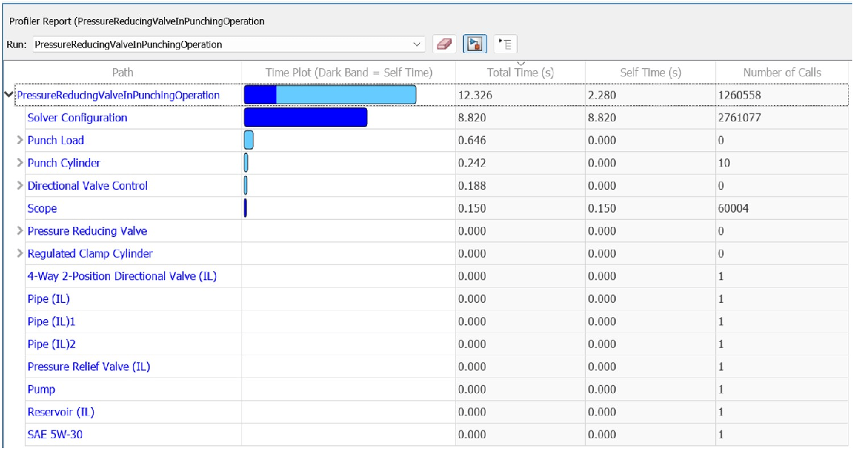
When simulation is complete, the Profiler Report pane displays the simulation profile for the model. Expand PressureReducingValveInPunchingOperation. By default, the profiler sorts the blocks at the same level of the model in descending order by the values in the Total Time(s) column. The contribution of the Simscape blocks is grouped in the Solver Configuration row. Although the Simscape blocks take up the most time (8.82 s) out of the total time (12.326 s), the time consumed by the Simulink blocks can be minimized. The Punch Load subsystem takes up the most time (0.646 s), followed by the Punch Cylinder subsystem (0.242 s) and the Directional Valve Control subsystem (0.188 s). Additionally, logging the results to the Scope block leads to a slowdown of 0.15 s. Expand the subsystems hierarchy to see how much time each block takes up.

You can see that within Punch Load subsystem, the blocks such as Switch and Saturation lead to minor slowdown due to their non-linear behavior. The execution of these subsystems can be sped up by implementing these steps:

Convert the Punch Load and Directional Valve Control subsystems to Atomic Subsystems with a higher sample time. The subsystems named Punch Load and Directional Valve Control are virtual subsystems. Virtual subsystems are treated as if all the blocks existed at the same level. Atomic subsystems let you control the execution of the model. Right click on the subsystems, then click Block Parameters (subsystem). Enable the Treat as atomic unit option and set the Sample time to 1e-3, that is higher than the sample time of the local solver (1e-4) so that the blocks of the subsystem run faster.

Add Rate Transition blocks at the input and output of the subsystems. The Rate Transition block transfers data from the output of a block operating at one rate to the input of a block operating at a different rate. Use the block parameters to ensure data integrity and deterministic transfer for faster response or lower memory requirements.

Run the model again and check if the simulation time has improved.

simIn = Simulink.SimulationInput(model);
simIn = setModelParameter(simIn,'StopTime','6');
out = sim(simIn);
simMetadata = getSimulationMetadata(out);
simMetadata.TimingInfo;
simMetadata.TimingInfo.ExecutionElapsedWallTime;

You can also run the Performance Advisor to automatically fix performance-related issues in the model. To open the Performance Advisor, on the Debug tab, click the Performance button arrow and select Performance Advisor. To learn more, see Improve Simulation Performance Using Performance Advisor.

Configure the Model

You can configure the model to experience further improvement in speed.

• Modify or Remove Elements that Create Discontinuities

A valve with zero smoothing factor causes discontinuities during near-open and near-closed positions. These discontinuities cause the solver to take smaller time steps and slows the simulation down. A non-zero smoothing factor implements a piecewise quadratic smoothing function that helps avoid these discontinuities during near-open and near-closed positions. A higher value of smoothing factor increases the effect of the smoothing function.

The 4-Way 2-Position Directional Valve and the Check Valve blocks have their Smoothing factor parameters set to 0.01. Set the Smoothing factor parameter of these blocks to 0.1 to observe a slight improvement in simulation speed.

set_param([model '/4-Way 2-Position Directional Valve (IL)'],'smoothing_factor','0.1');
set_param([model '/Pressure Reducing Valve/Check Valve'],'smoothing_factor','0.1');

• Modify or Remove Elements with Small Time Constant

The Pipe (IL) blocks in the model have the Fluid dynamic compressibility parameter set to On. When dynamic compressibility is on, an imbalance of mass inflow and mass outflow can cause liquid to accumulate or diminish in the pipe. As a result, pressure in the pipe volume can rise and fall dynamically, which provides some compliance to the system and modulates rapid pressure changes. These pressure changes increase the model complexity and the simulation time. Also, the pipe friction can induce discontinuities.

Remove the Pipe (IL), Pipe (IL)1 and Pipe (IL)2 blocks. To compensate for the pipe volume, increase the dead volume of the single-acting actuators that represent the punch cylinder, clamp cylinder and pressure reducing valve spool. Navigate inside Punch Cylinder subsystem. Increase the value of Dead volume in chamber A and Dead volume in chamber B parameters of the Punch Cylinder block from 1e-6 m^3 to 1e-3 m^3. Navigate inside Regulated Clamp Cylinder subsystem. Increase the value of Dead volume in chamber A and Dead volume in chamber B parameters of the Clamp Cylinder block from 1e-6 m^3 to 1e-3 m^3. Navigate inside Pressure Reducing Valve subsystem. Increase the value of Dead volume parameter of the Single-Acting Actuator (IL) and Single-Acting Actuator (IL)1 blocks from 1e-5 m^3 to 1e-4 m^3. These changes lead to an improvement in speed with no marked difference in the results.

set_param([model '/Punch Cylinder/Punch Cylinder'],'dead_volume_A','1e-3');
set_param([model '/Punch Cylinder/Punch Cylinder'],'dead_volume_B','1e-3');
set_param([model '/Regulated Clamp Cylinder/Clamp Cylinder'],'dead_volume_A','1e-3');
set_param([model '/Regulated Clamp Cylinder/Clamp Cylinder'],'dead_volume_B','1e-3');
set_param([model '/Pressure Reducing Valve/Single-Acting Actuator (IL)'],'dead_volume','1e-4');
set_param([model '/Pressure Reducing Valve/Single-Acting Actuator (IL)1'],'dead_volume','1e-4');

Now you can close the original model.

bdclose(model)
bdclose all

Simulate the Real-Time Model

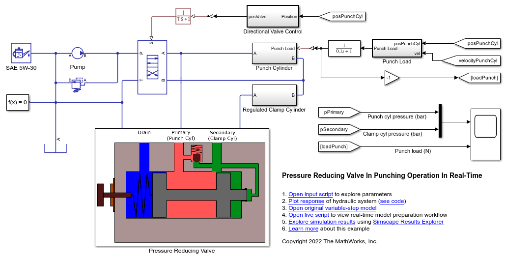
Open the PressureReducingValveInRealTime model, that is already optimized for real-time simulation.

modelRT = 'PressureReducingValveInRealTime';
open_system(modelRT)

Open the Configuration Parameters window, click Data Import/Export, then enable the Single simulation output parameter to return simulation data as a single Simulink.SimulationOutput object and set the object name to out_PressureReducingValveInRealTime.

set_param(modelRT,'ReturnWorkspaceOutputs','on');
set_param(modelRT,'ReturnWorkspaceOutputsName','out_PressureReducingValveInRealTime');

Set Simulation stop time (sec) to 6.

set_param(modelRT,'StopTime','6');

Enable the Use local solver option in the Solver Configuration block. Set Solver type to Backward Euler and Sample time to 2e-4. Enable the Use fixed-cost runtime consistency iterations option in the Solver Configuration block. Expand the Use fixed-cost runtime consistency iterations option and set Nonlinear iterations to 3.

solverConfigurationRT = string(find_system(bdroot,'MaskType','Solver Configuration'));
set_param(solverConfigurationRT,'UseLocalSolver','on');
set_param(solverConfigurationRT,'LocalSolverChoice','NE_BACKWARD_EULER_ADVANCER');
set_param(solverConfigurationRT,'LocalSolverSampleTime','2e-4');
set_param(solverConfigurationRT,'DoFixedCost','on');
set_param(solverConfigurationRT,'MaxNonlinIter','3');

Open the Configuration Parameters window, click Solver, under Solver selection, set Type to Fixed-step, set Solver to ode1be (Backward Euler), and under Solver details, set Fixed-step size to 2e-4.

set_param(modelRT,'SolverType','Fixed-step');
set_param(modelRT,'SolverName','ode1be');
set_param(modelRT,'FixedStep','2e-4');

Create a Simulink.SimulationInput object with Simulation stop time (sec) as an input argument. Specify a Simulink.SimulationOutput object. Run the model optimized for real-time simulation.

simIn = Simulink.SimulationInput(modelRT);
simIn = setModelParameter(simIn,'StopTime','6');
out_PressureReducingValveInRealTime = sim(simIn);

After running the model, access the metadata and the timing information.

simMetadata = getSimulationMetadata(out_PressureReducingValveInRealTime);
simMetadata.TimingInfo;

To view the elapsed simulation time, in seconds, enter:

simMetadata.TimingInfo.ExecutionElapsedWallTime;

The elapsed run time is less than the simulation time, that indicates the model runs faster than real-time.

Generate and Build Code

After you optimize the model for real-time simulation, you can generate code from the model and build the code.

• Generate Code from the Model

To generate code from the real-time model

1. In the Modeling tab, click Model Settings. The Configuration Parameters dialog opens. Navigate to the Code Generation tab, under Build process, select the Generate code only parameter, and click Apply.

2. Note that the system target file must be grt.tlc. In the Configuration Parameters window, click Code Generation. In the right pane, set System Target File to grt.tlc.

3. In the Apps tab, under Code Generation, click Simulink Coder. In the C Code tab, click Generate Code.

After the model finishes generating code, a new subfolder called PressureReducingValveInRealTime_grt_rtw is created in your current MATLAB working folder and the Code Generation Report window opens. This subfolder contains the files created by the code generation process, including those that contain the generated C source code.

• Build the Generated Code

To build an executable, you must set up a supported C/ C++ compiler. For a list of compilers supported in the current release, see Supported and Compatible Compilers.

To set up your compiler, run this command in the MATLAB command prompt: mex -setup

After you set up your compiler, you can build and run the compiled code. The PressureReducingValveInRealTime model is currently configured to only generate code. To build the generated code:

1. In the Modeling tab, click Model Settings. The Configuration Parameters dialog opens. Click Code Generation, then clear the Generate code only parameter and click Apply.

2. In the C Code tab, click Build.

The code generator builds the executable and generates the Code Generation Report. The code generator places the executable in the working folder. The executable generated is PressureReducingValveInRealTime.exe.

You can run the generated executable from MATLAB command prompt with this command to create a MAT-file that contains the same variables as those generated by simulating the model.

% !PressureReducingValveInRealTime

clear all
close all
bdclose all