Hydraulic Actuator with Telescopic Cylinder

Open Live Script

This example demonstrates the extension and retraction of a telescopic hydraulic actuator with three stages. The telescopic actuator extends and retracts one stage at a time.

Model

The model represents an actuator controlled by a 3-way, 2-position valve. As the control signal acts on the valve, the actuator chamber connects to the pump, and the actuator begins to extend. An external load retracts the actuator when the valve connects the chamber to the tank. The set pressure differential of the pressure relief valve is 50 bar, and the applied load is 2100 N.

open_system('HydraulicActuatorWithTelescopicCylinder');

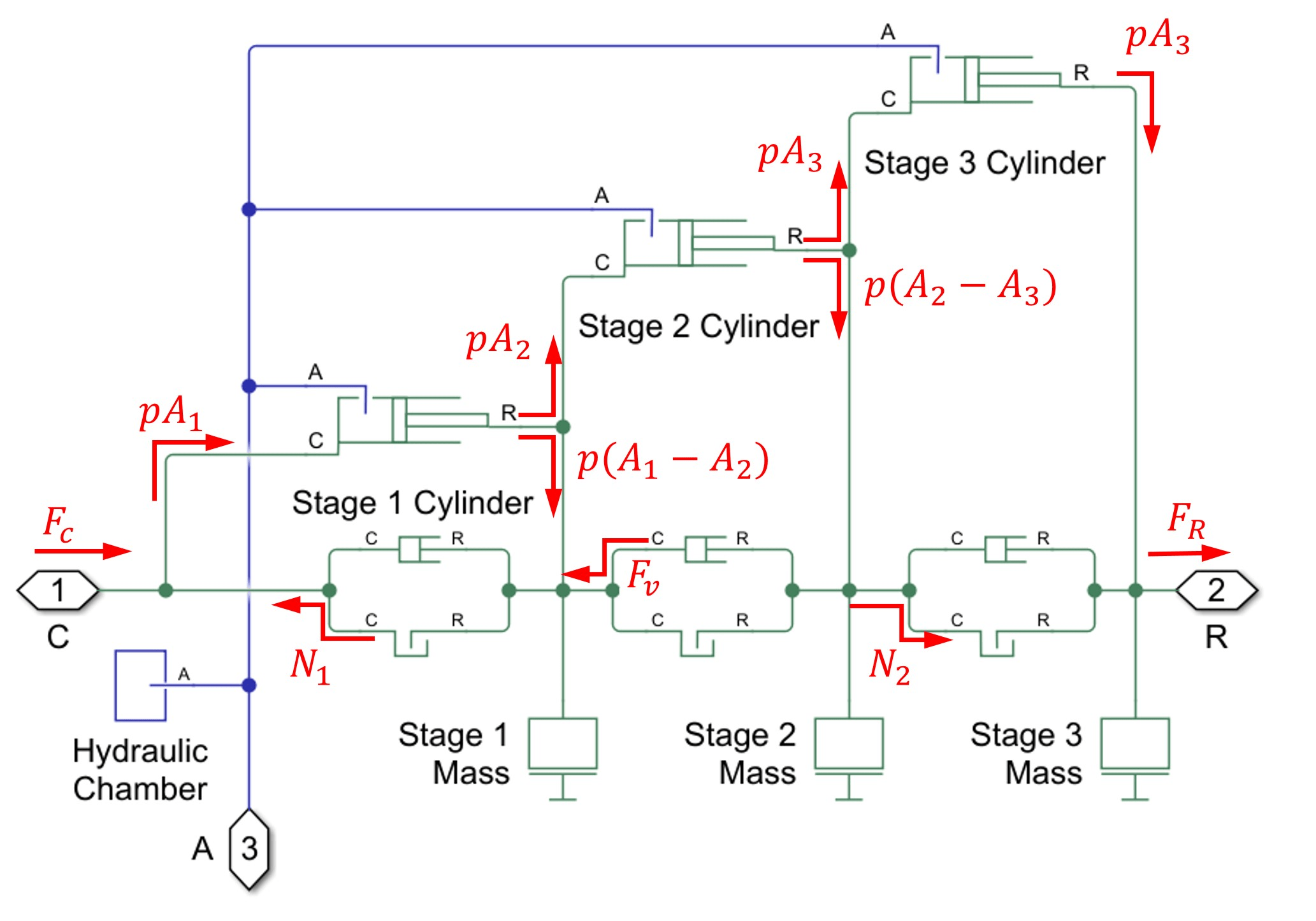
Telescopic Cylinder Subsystem

A Translational Mechanical Converter (IL) block represents each stage. The mechanical converter blocks are connected in series. A stage interacts with neighboring stages through hard stops and viscous forces.

open_system('HydraulicActuatorWithTelescopicCylinder/Telescopic Cylinder');

This figure shows a physical diagram of the cylinder.

The effective areas of the stages are $A_{1} = 20$ , $A_{2} = 16$ , and $A_{3} = 12 c m^{2}$ , respectively, and the mass of each stage is $6.4 k g$ .

Cylinder Pressure and Stage Extensions

Plot the cylinder pressure and stage extensions.

HydraulicActuatorWithTelescopicCylinderPlot1Cyl;

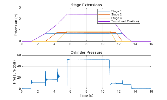
Figure HydraulicActuatorWithTelescopicCylinder contains 2 axes objects. Axes object 1 with title Stage Extensions, ylabel Extension (m) contains 4 objects of type line. These objects represent Stage 1, Stage 2, Stage 3, Sum (Load Position). Axes object 2 with title Cylinder Pressure, xlabel Time (s), ylabel Pressure (bar) contains an object of type line.

The cylinder extends and retracts each stage sequentially. This behavior happens because the stages are subject to the same fluid pressure $p$ while having different effective areas $A_{1}, A_{2}, A_{3}$ . For example, when the first stage extends or retracts, its force $p A_{1}$ is sufficient to bear the external load, whereas the forces of the subsequent stages are not.

Force Balances

These free body diagrams illustrate the forces acting on different parts of the cylinder during the period when the second stage extends with a constant velocity.

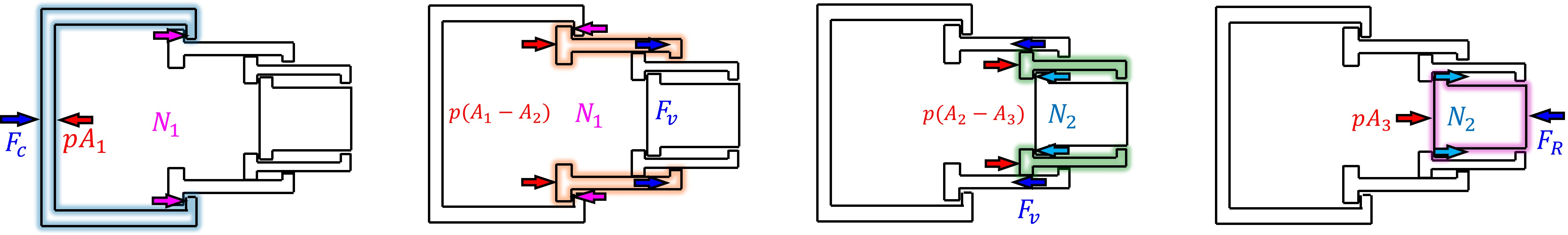
From left to right, the following equations hold.

$F_{c} + N_{1} = p A_{1}$

$p (A_{1} - A_{2}) + F_{v} = N_{1}$

$p (A_{2} - A_{3}) = N_{2} + F_{v}$

$p A_{3} + N_{2} = F_{R}$

where $F_{c}$ and $F_{R}$ are the forces at port C and R, respectively, and $N$ represents a hard-stop force, and $F_{v}$ is the viscous force associated to the movement of the second stage. The sum of all equations gives $F_{c} = F_{R}$ . The diagram shows how the forces on the free body diagrams manifest across the network.

In the force flow diagram, when a force flows from a block port into a node at a network junction, it indicates that the block is applying force to the node. Conversely, when a force flows from the node into a block, it represents that the node is applying force to the block. The force flows on the diagram can be verified using the simulation log or placing Ideal Force Sensor blocks. For example, verify the second equation $p (A_{1} - A_{2}) + F_{v} = N_{1}$ .

pA1 = -simlog_HydraulicActuatorWithTelescopicCylinder.Telescopic_Cylinder.Stage_1_Cylinder.interface_force.series.values('N'); % p*A_1 (N) 
pA2 = -simlog_HydraulicActuatorWithTelescopicCylinder.Telescopic_Cylinder.Stage_2_Cylinder.interface_force.series.values('N'); % p*A_2 (N)
Fv = simlog_HydraulicActuatorWithTelescopicCylinder.Telescopic_Cylinder.Stage_2_Damper.f.series.values('N');                   % F_v (N)
N1 = simlog_HydraulicActuatorWithTelescopicCylinder.Telescopic_Cylinder.Stage_1_Hard_Stop.f.series.values('N');                % N_1 (N)
time = simlog_HydraulicActuatorWithTelescopicCylinder.Telescopic_Cylinder.Stage_1_Cylinder.interface_force.series.time;        % Time (s)
forceResidual = pA1 - pA2 + Fv - N1;                                                                                           % Residual of equation (N)
figure, plot(time, [pA1, pA2, Fv, N1, forceResidual], 'LineWidth', 1);
xlim([3 4]);
xlabel('Time (s)');
ylim([-500 4000]);
ylabel('Force (N)');
legend('$pA_1$','$pA_2$','$F_v$','$N_1$','$pA_1-pA_2+F_v-N_1$','Interpreter','latex');

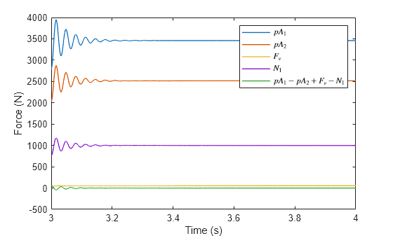
Figure contains an axes object. The axes object with xlabel Time (s), ylabel Force (N) contains 5 objects of type line. These objects represent $pA_1$, $pA_2$, $F_v$, $N_1$, $pA_1-pA_2+F_v-N_1$.

The oscillations are caused by the hard-stop dynamics that generate $N_{1}$ . Once the oscillations decay, the equation holds.

Hydraulic Actuator with Telescopic Cylinder

Model

Telescopic Cylinder Subsystem

Cylinder Pressure and Stage Extensions

Force Balances

See Also