Simulate Multivariate Markov-Switching Dynamic Regression Model
This example shows how to generate random response and state paths from a two-state Markov-switching dynamic regression model.
Consider the response processes and that switch between three states, governed by the latent process with this observed transition matrix:
Suppose that is a VARX model in each state:
where, for j = 1,2,3, is Gaussian with mean 0 and covariance matrix
Create Fully Specified Model
Create the Markov-switching dynamic regression model that describes and .
% Switching mechanism
P = [10 1 1; 1 10 1; 1 1 10];
mc = dtmc(P);

% VAR submodels
C1 = [1;-1];
C2 = [2;-2];
C3 = [3;-3];
AR1 = {};
AR2 = {[0.5 0.1; 0.5 0.5]};
AR3 = {[0.25 0; 0 0] [0 0; 0.25 0]};
Beta1 = [1; -1];
Beta2 = [2 2;-2 -2];
Beta3 = [3 3 3;-3 -3 -3];
Sigma1 = [1 -0.1; -0.1 1];
Sigma2 = [2 -0.2; -0.2 2];
Sigma3 = [3 -0.3; -0.3 3];
mdl1 = varm(Constant=C1,AR=AR1,Beta=Beta1,Covariance=Sigma1);
mdl2 = varm(Constant=C2,AR=AR2,Beta=Beta2,Covariance=Sigma2);
mdl3 = varm(Constant=C3,AR=AR3,Beta=Beta3,Covariance=Sigma3);

Mdl = msVAR(mc,[mdl1; mdl2; mdl3]);
Mdl is a fully specified msVAR object.
Simulate One Path
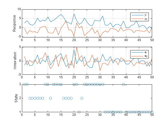
Simulate one path of responses, innovations, and state indices from the model. Specify a 50-period simulation horizon, that is, a 50-observation path for all variables.
rng("default") % For reproducibility
numObs = 50;
[Y,E,SP] = simulate(Mdl,numObs);
Y and E are 50-by-2 vectors of simulated responses and innovations, respectively. SP is a 50-by-1 vector of state indices. By default, simulate ignores the regression components.
Plot the results in separate subplots.
figure
tiledlayout(3,1)
nexttile
plot(Y)
ylabel("Response")
grid on
legend("y_1","y_2")

nexttile
plot(E)
ylabel("Innovation")
grid on
legend("e_1","e_2")

nexttile
plot(SP,"o")
ylabel("State")
yticks([1 2 3])
Simulate Multiple Paths
Simulate three separate, independent paths of responses and state indices from the model. Specify a 5-period simulation horizon.
[Y3,~,SP3] = simulate(Mdl,5,NumPaths=3)
Y3 =
Y3(:,:,1) =

    4.5327   -4.3488
    1.9558   -5.7975
    1.9899   -4.2143
    3.1917   -1.9057
    5.1687   -1.9652


Y3(:,:,2) =

    4.6388   -1.9800
    3.9371   -0.0119
    4.2272   -1.2576
    3.3144   -0.9191
    4.7844   -0.1464


Y3(:,:,3) =

    5.4695   -0.4217
    3.1120    0.3758
    5.3764   -0.8609
    5.4875   -2.2966
    4.2543   -1.5557
SP3 = 5×3

     3     2     2
     3     2     2
     3     2     2
     3     2     3
     3     2     3
Y is a 5-by-2-by-3 array of simulated responses. SP is a 5-by-3 matrix of simulated state indices.
The simulated observation of in the second period of the first path is 1.9558.
The simulated observation of in the second period of the first path is 3.9371.
The corresponding simulated state in the second period of the first path is in state 3.
Simulate Model Containing Regression Component
simulate requires exogenous data over the simulation horizon for the regression component. Generate a 50-by-3 matrix of iid standard normal observations for the required exogenous data.
Pred = randn(numObs,3);
Simulate one path of responses, innovations, and state indices from the model. Specify a 50-period simulation horizon. Plot the results. To determine how the response and state paths compare to the model without regression components, reset the random seed to default.
rng("default")
[YReg,EReg,SPReg] = simulate(Mdl,numObs,X=Pred);

figure
tiledlayout(3,1)
nexttile
plot([Y YReg])
ylabel("Response")
grid on
legend("y_1","y_2","yreg_1","yreg_2")

nexttile
plot([E EReg])
ylabel("Innovation")
grid on
legend("e_1","e_2","ereg_1","ereg_2")

nexttile
plot(1:numObs,SP,"r.",1:numObs,SPReg,"ko")
ylabel("State")
legend("sp","spreg")
yticks([1 2 3]);

Innovations and state paths are equivalent between models, but response paths differ.