Select ARCH Lags for GARCH Model Using Econometric Modeler App
This example shows how to select the appropriate number of ARCH
and GARCH lags for a GARCH model by using the Econometric Modeler app. The data set,
stored in Data_MarkPound, contains daily Deutschmark/British
pound bilateral spot exchange rates from 1984 through 1991.
Import Data into Econometric Modeler
At the command line, load the Data_MarkPound.mat data
set.
load Data_MarkPoundAt the command line, open the Econometric Modeler app.
econometricModeler
Alternatively, open the app from the apps gallery (see Econometric Modeler).
Import Data to the app:
On the Modeler tab, in the Import section, click
 .
.In the Import Data dialog box, select the check box for the Data variable.
Click Import.
The variable Data1 appears in the Time
Series pane, and its time series plot appears in the
Plot(Data1) figure window.
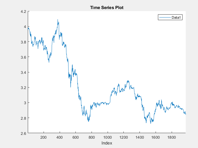
The exchange rate looks nonstationary (it does not appear to fluctuate around a fixed level).
Transform Data
Convert the exchange rates to returns.
With
Data1selected in the Time Series pane, on the Modeler tab, in the Transforms section, click Log.In the Time Series pane, a variable representing the logged exchange rates (
Data1_Log) appears , and its time series plot appears in the Plot(Data1_Log) figure window.In the Time Series pane, select
Data1_Log.On the Modeler tab, in the Transforms section, click Difference.
In the Time Series pane, a variable representing the
returns (Data1_Log_Diff) appears. A time series plot
of the differenced series appears in the
Plot(Data1_Log_Diff) figure window.
Check for Autocorrelation
In the Time Series pane, rename the
Data1_Log_Diff variable by clicking it twice to
select its name and entering Returns.
The app updates the names of all documents associated with the returns.
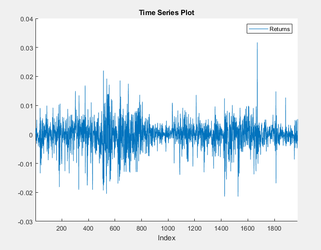
The returns series fluctuates around a common level, but exhibits volatility clustering. Large changes in the returns tend to cluster together, and small changes tend to cluster together. That is, the series exhibits conditional heteroscedasticity.
Visually assess whether the returns have serial correlation by plotting the sample ACF and PACF:
Close all figure windows in the right pane.
In the Time Series pane, select the
Returnstime series.Click the Plots tab, then click ACF.
Click the Plots tab, then click PACF.
Drag the PACF(Returns) figure window below the ACF(Returns) figure window so that you can view them simultaneously.
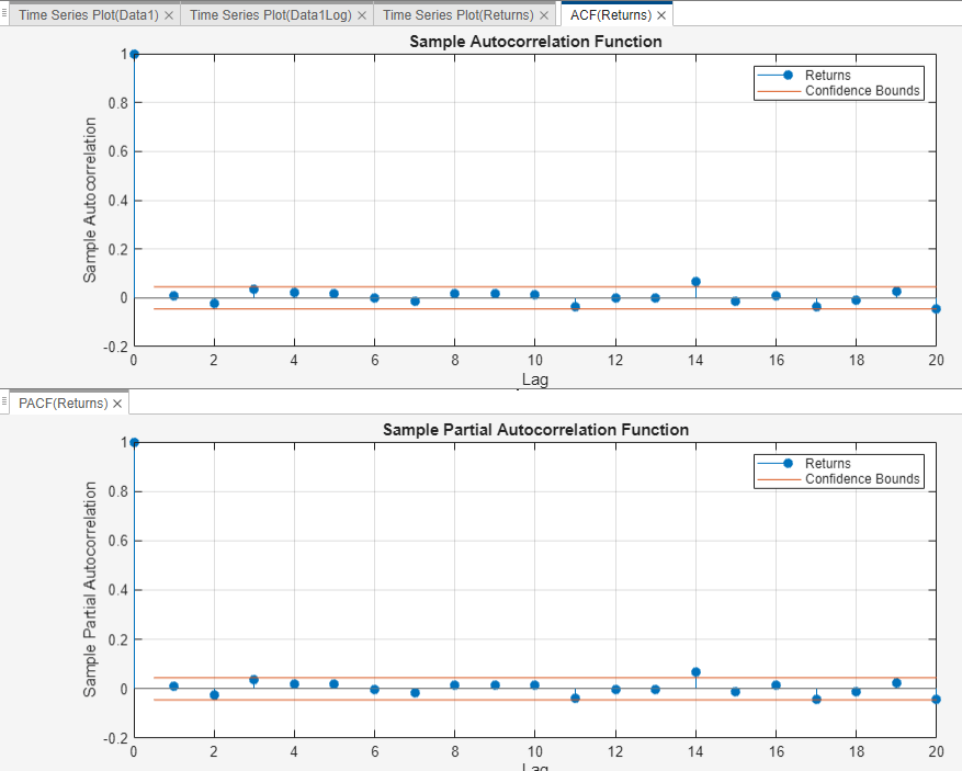
The sample ACF and PACF show virtually no significant autocorrelation.
Conduct the Ljung-Box Q-test to assess whether there is significant serial correlation in the returns for at most 5, 10, and 15 lags. To maintain a false-discovery rate of approximately 0.05, specify a significance level of 0.05/3 = 0.0167 for each test.
Close the ACF(Returns) and PACF(Returns) figure windows.
With
Returnsselected in the Time Series pane, on the Modeler tab, in the Tests section, click Add Test > Ljung-Box Q-Test.On the LBQ tab, in the Settings section, set Number of Lags to
5. The DOF setting changes to5.Set Significance Level to
0.0167.In the Tests section, click Run Test.
Repeat steps 3 through 5 twice, with these changes.
Set Number of Lags to 10 and the DOF to 10.
Set Number of Lags to 15 and the DOF to 15.
The test results appear in the Results table of the LBQ(Returns) document.
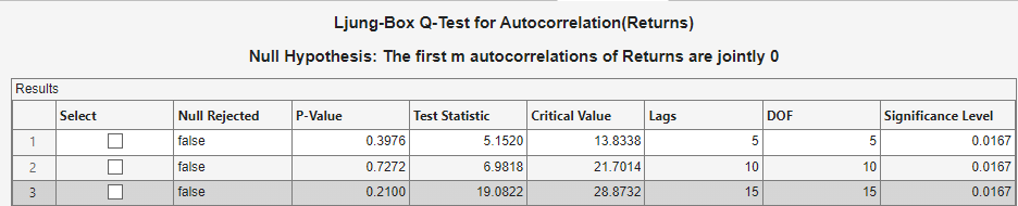
The Ljung-Box Q-test null hypothesis that all autocorrelations up to the tested lags are zero is not rejected for tests at lags 5, 10, and 15. These results, and the ACF and PACF, suggest that a conditional mean model is not needed for this returns series.
Check for Conditional Heteroscedasticity
Check the returns for conditional heteroscedasticity by plotting the ACF and PACF of the demeaned, squared returns. Then, determine the appropriate number of lags for a GARCH model of the returns by conducting Engle's ARCH test on the demeaned returns.
Compute the series of squared residuals at the command line by demeaning the returns, then squaring each element of the result.
Export Returns to the command line:
In the Time Series pane, right-click
Returns.In the context menu, select
Export.
Returns appears in the MATLAB® Workspace.
Remove the mean from the returns, then square each element of the result. To
ensure all series in the Time Series pane are synchronized,
Econometric Modeler prepends first-differenced series with a
NaN value. Therefore, to estimate the sample mean, use
mean(Returns,"omitnan").
Residuals = Returns - mean(Returns,"omitnan");
Residuals2 = Residuals.^2;
Create a table containing the Returns and
Residuals2 variables.
Tbl = table(Returns,Residuals,Residuals2);
Import Tbl into Econometric Modeler:
On the Modeler tab, in the Import section, click
.The app must clear the right pane and all documents before importing new data. Therefore, after clicking Import, in the Econometric Modeler dialog box, click Yes.
In the Import Data dialog box, select the check box for the Tbl variable.
Click Import.
The variables appear in the Time Series pane, and a time series plot of all the series appears in the Plot(Residuals) figure window.
Plot the ACF and PACF of the squared residuals.
Close the Plot(Residuals) figure window.
In the Time Series pane, select the
Residuals2time series.Click the Plots tab, then click ACF.
Click the Plots tab, then click PACF.
Drag the PACF(Residuals2) figure window below the ACF(Residuals2) figure window so that you can view them simultaneously.

The sample ACF and PACF of the squared returns show significant autocorrelation. This result suggests that a GARCH model with lagged variances and lagged squared innovations might be appropriate for modeling the returns.
Conduct Engle's ARCH test on the residuals series. Specify a two-lag ARCH model alternative hypothesis.
Close all figure windows.
In the Time Series pane, select the
Residualstime series.On the Modeler tab, in the Tests section, click Add Test > Engle's ARCH Test.
On the ARCH tab, in the Settings section, set Number of Lags to
2.In the Tests section, click Run Test.
The test results appear in the Results table of the ARCH(Residuals) document.

Engle's ARCH test rejects the null hypothesis of no ARCH effects in favor of the alternative ARCH model with two lagged squared innovations. An ARCH model with two lagged innovations is locally equivalent to a GARCH(1,1) model.
Create and Fit GARCH Model
Fit a GARCH(1,1) model to the returns series.
In the Time Series pane, select the
Returnstime series.Click the Modeler tab. Then, in the Models section, click the arrow to display the models gallery.
In the models gallery, in the GARCH Models section, click GARCH.
In the GARCH Model Parameters dialog box, on the Lag Order tab, observe that the ARCH and GARCH orders are 1 by default, and the model includes an offset, which is required when the series is not centered at zero.
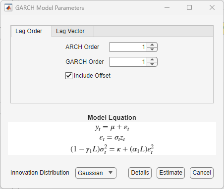
Click Estimate.
The model variable GARCH_Returns appears in the
Models pane, its value appears in the
Preview pane, and its estimation summary appears in the
Fit(GARCH_Returns) document.
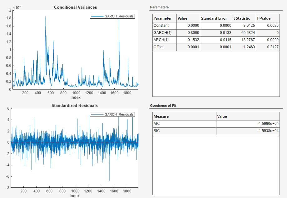
An alternative way to select lags for a GARCH model is by fitting several models containing different lag polynomial degrees. Then, choose the model yielding the minimal AIC.