Operate on Variables In Econometric Modeler

This topic shows you how to determine which variable is active in Econometric Modeler, which operations are available for the active variable, and how to know which variable will be active after you apply an operation.

Active Variable Operations

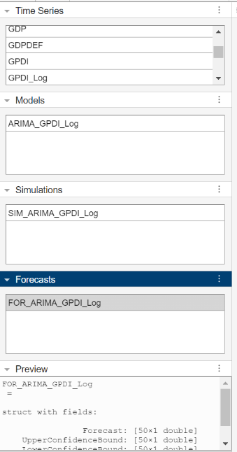
Econometric Modeler enables you to plot, conduct statistical tests, and transform imported time series variables, among other operations. Some operations create new variables, plots, and operation-summary documents, for example, when you apply the log transform to a time series, Econometric Modeler creates a new time series variable representing the transformation and it shows a plot of the transformation in a new document. When you fit a model to time series data, Econometric Modeler creates a model object representing the estimated model and shows an estimation summary in a new document. New variables appear in the associated section in the left pane, for example, new variables of transformed time series appear in the Time Series pane, and new estimated models appear in the Models pane. This figure shows the contents of the left pane.

As you work in Econometric Modeler, the active variable might change. Active variables are highlighted in the left pane, Econometric Modeler applies operations, on which you click, to the active variable. To make a different variable active, click that variable at any time. If you double-click a variable, the variable is active and a document containing its plot or operation summary appears in the right pane. When you make a different variable active or apply an operation to an active variable, you might see operations on the active tab deactivate (gray out) or become available. This behavior occurs because Econometric Modeler switches the context of the app to focus on operations that apply to the new active variable.

This table shows which operations are available for each variable type, what type of variable is created after you apply an operation, and which variable is active after the operation is applied.

Active Variable(s)	Operation	Active Variable After Operation
One time series in the Time Series pane	Generate single-variable plot by clicking, on the Plots tab, Time Series, ACF, or PACF.	Same time series
	Conduct single-variable hypothesis test by clicking Add Test, and then selecting any test in the Stationarity, Heteroscedasticity, or Autocorrelation section.	Same time series
	Transform the time series by clicking, in the Transforms section, any transformation.	In the Time Series pane, the transformed variable
	Apply a business cycle filter to the time series by clicking, in the Filters section, Filter Data, and then any business cycle filter.	In the Time Series section, variables representing the cyclical and trend components (two new variables, both are active)
	Estimate an univariate model by clicking the arrow in the Models section, and selecting any model in the ARIMA, GARCH, and Regression Models section.	In the Models pane, the estimated model
At least one time series in the Time Series pane	Generate plot by clicking, on the Plots tab, Time Series, Y-Y Axis (for two time series), or Corr.	Same time series
	Conduct multivariate hypothesis test by clicking Add Test, and then selecting any test in the Collinearity or Cointegration section.	Same time series
	Transform time series by clicking, in the Transforms section, any transformation.	In the Time Series pane, the transformed variables
	Apply a business cycle filter to time series by clicking, in the Filters section, Filter Data, and then any business cycle filter.	In the Time Series section, variables representing the cyclical and trend components (two new variables per filtered time series, both become active)
	Estimate a multivariate model by clicking the arrow in the Models section, and selecting any model in the Multivariate Models section.	In the Models pane, the estimated model
One model in the Models pane	Plot the model's fitted values or a residual plot by clicking, on the Plots tab, any available plot.	Same estimated model
	Conduct model residual hypothesis test by clicking Add Test, and then selecting any test in the Model Residuals section.	Same estimated model
	Perform model diagnostics by clicking, in the Diagnostics section, Model Fit Diagnostics, and then selecting any model diagnostic in the menu.	Same estimated model
	Simulate in-sample model response paths by clicking, in the Simulate section, Simulate.	In the Simulations pane, the simulated paths and confidence interval bounds (one variable)
	Forecast model responses by clicking, in the Forecast section, Forecast.	In the Forecasts pane, the forecasted responses and forecast interval bounds (one variable)
One model simulation in the Simulations pane	No available operation	Not applicable
One series of model forecasts in the Forecast pane	No available operation	Not applicable

Note

After you simulate or forecast an estimated model, all operations, except for session export options in the Export section, are unavailable. Click a time series, in the Time Series pane, or an estimation model, in the Models pane, to continue working in Econometric Modeler.

Track Active Variable in Econometric Modeler

This example shows how to estimate a VAR model, and then generate forecasts from the model by using the Econometric Modeler app. The example highlights which variable is active after each operation.

The data set, which is stored in Data_USEconModel.mat, contains the raw, quarterly US GDP, M1 money supply, and 3-month T-bill rate, among other series, from 1947 through 2009.

Load and Import Data into Econometric Modeler

At the command line, load the Data_USEconModel.mat data set.

load Data_USEconModel

At the command line, open the Econometric Modeler app.

econometricModeler

Alternatively, open the app from the apps gallery (see Econometric Modeler).

Import DataTimeTable into the app:

1. On the Modeler tab, in the Import section, click the Import button .

2. In the Import Data dialog box, select the check box for the DataTimeTable variable.

3. Click Import.

GDP, M1SL, and TB3MS, among other series, appear in the Time Series pane, and a time series plot containing all series appears in the figure window. Because all time series are selected, all are active.

Transform Series

Remove the exponential trend from the GDP and M1 money supply series by applying the log transform to each series. Click the Modeler tab, and then, in the Time Series pane, click GDP and Ctrl click M1SL. In the Transforms section, click Log. The transformed series GDP_Log and M1SL_Log appear in the Time Series pane; these two variables are the only selected variables, therefore, they are active.

Stabilize the series by applying the first difference to each series.

1. Click the Modeler tab, and then, in the Time Series pane, click GDP_Log and Ctrl+click M1SL_Log and TB3MS.

2. In the Transforms section, click Difference. The transformed series GDP_Log_Diff, M1SL_Log_Diff, and TB3MS_Diff appear in the Time Series pane. The three new variables are active.

3. Rename GDP_Log_Diff and M1SL_Log_Diff to GDPRate and M1SLRate by clicking their names twice in the Time Series pane, and typing their new names. The last variable you rename is the only active variable.

Estimate VAR Models

Fit a 3-D VAR(2) model to the US quarterly GDP growth rate series GDPRate, M1 money supply growth rate series M1SLRate, and change in the 3-month treasury bill rate series TB3MS_Diff.

1. In the Time Series pane, click GDPRate and Ctrl+click M1SLRate and TB3MS_Diff. These three variables are active.

2. In the Models section, click VAR.

3. In the VAR Model Parameters dialog box, set Autoregressive Order (p) to 2. Then, click Estimate.

   The model variable VAR appears in the Models pane, its value appears in the Preview pane, and its estimation summary appears in the Fit(VAR) document. The estimated VAR(2) model VAR is the active variable.

Forecast Estimated Model

Forecast the model into a 10-year (40-period) horizon.

1. In the Models pane, select the VAR model.

2. On the Modeler tab, in the Forecast section, click Forecast.

3. In the Forecast Model Response dialog box, set Number of periods in forecast horizon to 40. Click Forecast.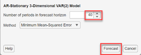

   

In the Forecasts pane, a variable For_VAR appears and is active. Note that all operations are unavailable, except for export options.