Estimate Random Parameter of State-Space Model
This example shows how to estimate a random, autoregressive coefficient of a state in a state-space model. That is, this example takes a Bayesian view of state-space model parameter estimation by using the "zig-zag" estimation method.
Suppose that two states ( and ) represent the net exports of two countries at the end of the year.
is a unit root process with a disturbance variance of .
is an AR(1) process with an unknown, random coefficient and a disturbance variance of .
An observation () is the exact sum of the two net exports. That is, the net exports of the individual states are unknown.
Symbolically, the true state-space model is
Simulate Data
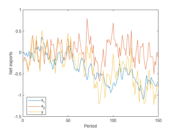
Simulate 100 years of net exports from:
A unit root process with a mean zero, Gaussian noise series that has variance .
An AR(1) process with an autoregressive coefficient of 0.6 and a mean zero, Gaussian noise series that has variance .
.
Create an observation series by summing the two net exports per year.
rng(100); % For reproducibility
T = 150;
sigma1 = 0.1;
sigma2 = 0.2;
phi = 0.6;

u1 = randn(T,1)*sigma1;
x1 = cumsum(u1);
Mdl2 = arima('AR',phi,'Variance',sigma2^2,'Constant',0);
x2 = simulate(Mdl2,T,'Y0',0);
y = x1 + x2;

figure;
plot([x1 x2 y])
legend('x_1','x_2','y','Location','Best');
ylabel('Net exports');
xlabel('Period');
The Zig-Zag Estimation Method
Treat as if it is unknown and random, and use the zig-zag method to recover its distribution. To implement the zig-zag method:
1. Choose an initial value for in the interval (-1,1), and denote it .
2. Create the true state-space model, that is, an ssm model object that represents the data-generating process.
3. Use the simulation smoother (simsmooth) to draw a random path from the distribution of the second smoothed states. Symbolically, .
4. Create another state-space model that has this form
In words, is a static state and is an "observed" series with time varying coefficient .
5. Use the simulation smoother to draw a random path from the distribution of the smoothed series. Symbolically, , where encompasses the structure of the true state-space model and the observations. is static, so you can just reserve one value ().
6. Repeat steps 2 - 5 many times and store each iteration.
7. Perform diagnostic checks on the simulation series. That is, construct:
Trace plots to determine the burn in period and whether the Markov chain is mixing well.
Autocorrelation plots to determine how many draws need removing to obtain a well-mixed Markov chain.
8. The remaining series represents draws from the posterior distribution of . You can compute descriptive statistics, or plot a histogram to determine the qualities of the distribution.
Estimate Random Coefficient Using Zig-Zag Method
Specify initial values, preallocate, and create the true state-space model.
phi0 = -0.3;             % Initial value of phi
Z = 1000;                % Number of times to iterate the zig-zag method
phiz = [phi0; nan(Z,1)]; % Preallocate

A = [1 0; 0 NaN];
B = [sigma1; sigma2];
C = [1 1];
Mdl = ssm(A,B,C,'StateType',[2; 0]);
Mdl is an ssm model object. The NaN acts as a placeholder for .
Iterate steps 2 - 5 of the zig-zag method.
for j = 2:(Z + 1);
    % Draw a random path from smoothed x_2 series.
    xz = simsmooth(Mdl,y,'Params',phiz(j-1));
    % The second column of xz is a draw from the posterior distribution of x_2.

    % Create the intermediate state-space model.
    Az = 1;
    Bz = 0;
    Cz = num2cell(xz((1:(end - 1)),2));
    Dz = sigma2;
    Mdlz = ssm(Az,Bz,Cz,Dz,'StateType',2);

    % Draw a random path from the smoothed phiz series.
    phizvec = simsmooth(Mdlz,xz(2:end,2));
    phiz(j) = phizvec(1);
    % phiz(j) is a draw from the posterior distribution of phi
end
phiz is a Markov chain. Before analyzing the posterior distribution of , you should assess whether to impose a burn-in period, or the severity of the autocorrelation in the chain.
Determine Quality of Simulation
Draw a trace plot for the first 100, 500, and all of the random draws.
vec = [100 500 Z];
figure;
for j = 1:3;
    subplot(3,1,j)
    plot(phiz(1:vec(j)));
    title('Trace Plot for \phi');
    xlabel('Simulation number');
    axis tight;
end
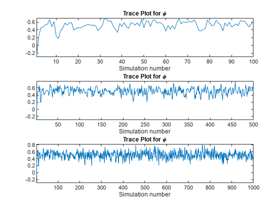
According to the first plot, transient effects die down after about 20 draws. Therefore, a short burn-in period should suffice. The plot of the entire simulation shows that the series settles around a center.
Plot the autocorrelation function of the series after removing the first 20 draws.
burnOut = 21:Z;

figure;
autocorr(phiz(burnOut));
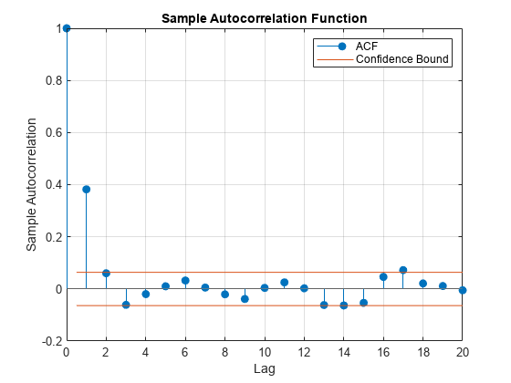
The autocorrelation function dies out rather quickly. It doesn't seem like autocorrelation in the chain is an issue.
Determine qualities of the posterior distribution of by computing simulation statistics and by plotting a histogram of the reduced set of random draws.
xbar = mean(phiz(burnOut))
xbar =
0.5104
xstd = std(phiz(burnOut))
xstd =
0.0988
ci = norminv([0.025,0.975],xbar,xstd); % 95% confidence interval

figure;
histogram(phiz(burnOut),'Normalization','pdf');
h = gca;
hold on;
simX = linspace(h.XLim(1),h.XLim(2),100);
simPDF = normpdf(simX,xbar,xstd);
plot(simX,simPDF,'k','LineWidth',2);
h1 = plot([xbar xbar],h.YLim,'r','LineWidth',2);
h2 = plot([0.6 0.6],h.YLim,'g','LineWidth',2);
h3 = plot([ci(1) ci(1)],h.YLim,'--r',...
    [ci(2) ci(2)],h.YLim,'--r','LineWidth',2);
legend([h1 h2 h3(1)],{'Simulation Mean','True Mean','95% CI'});
h.XTick = sort([h.XTick xbar]);
h.XTickLabel{h.XTick == xbar} = xbar;
h.XTickLabelRotation = 90;
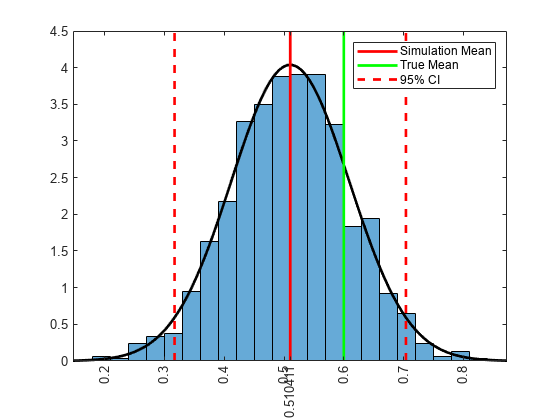
The posterior distribution of is roughly normal with mean and standard deviation approximately 0.51 and 0.1, respectively. The true mean of is 0.6, and it is less than one standard deviation to the right of the simulation mean.
Compute the maximum likelihood estimate of . That is, treat as a fixed, but unknown parameter, and then estimate Mdl using the Kalman filter and maximum likelihood.
[~,estParams] = estimate(Mdl,y,phi0)
Method: Maximum likelihood (fminunc)
Sample size: 150
Logarithmic  likelihood:     -10.1434
Akaike   info criterion:      22.2868
Bayesian info criterion:      25.2974
      |     Coeff       Std Err     t Stat       Prob
-------------------------------------------------------
 c(1) |  0.53590       0.19183    2.79360      0.00521
      |
      |   Final State   Std Dev    t Stat        Prob
 x(1) | -0.85059       0.00000   -6.45811e+08   0
 x(2) |  0.00454        0          Inf          0
estParams =
0.5359
The MLE of is 0.54. Both estimates are within one standard deviation or standard error from the true value of .
See Also
ssm | simulate | estimate | refine | simsmooth