Get Started with Underwater Acoustic Channels

R2026b

Since R2026b

The Underwater Acoustic Channels add-on provides functions for modeling an underwater acoustic environment and using MATLAB^® to interface with the Bellhop beam tracing model for simulating underwater sound propagation. The add-on includes these objects and functions:

• bellhopModel: Trace acoustic rays through a specified environment. Compute transmission loss over a region or multipath arrival at a receiver location using the transmissionLoss and propagationPaths object functions.

• bellhopConfiguration: Configure the path to a Bellhop executable, which you must install separately.

• underwaterSoundSpeed: Calculate sound speed profiles (SSPs) from temperature, salinity, and depth using established empirical equations (Mackenzie, Coppens, UNESCO/Chen-Millero, or Del Grosso).

• seaSurfaceHeight: Generate sea surface height realizations from standard wave spectra (Pierson-Moskowitz, JONSWAP, or Bretschneider).

To install the add-on, run installUWAChannels.

Model Underwater Acoustic Propagation Using Underwater Acoustic Channels

This example shows how to model underwater acoustic propagation using the Underwater Acoustic Channels add-on. You create environment models with different SSPs, surface conditions, and bathymetry, then compute transmission loss fields and eigenray arrival structures.

Configure Bellhop and Define Source Geometry

The bellhopModel object requires a Bellhop executable. If MATLAB is not currently configured to use Bellhop, uncomment the code below. Update the code with the path to your Bellhop executable and call bellhopConfiguration. You only need to do this once.

% Set the path to your Bellhop executable (required once per session).
% bellhopConfiguration(ExecutablePath="C:\path\to\bellhop.exe")

Create a bellhopModel object.

bh = bellhopModel;

Define a carrier frequency and source/receiver geometry.

fc = 500;
srcPos = [0; 0; 50];
rxPos = [0; 50000; 80];

Explore Effect of SSP on Propagation

The SSP, shaped by temperature, salinity, and pressure, controls ray refraction, creating phenomena such as surface shadow zones, deep sound channels, and convergence zones.

The default SSP in bellhopModel is the Munk canonical deep-ocean profile with a minimum speed at depth 1300 m. Create a baseline model and compute the transmission loss (TL) field. TL quantifies how much acoustic pressure decreases with range and depth due to geometric spreading, refraction, and absorption.

bh = bellhopModel;
bh.RayElevationAngles = [-30 30];
bh.RayTraceRangeLimit = 60000;
transmissionLoss(bh, fc, srcPos);

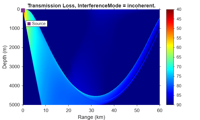
Sound speed increases with temperature and pressure but varies weakly with salinity. In a summer coastal environment, a warm surface layer over cold deep water (thermocline) causes sound speed to decrease with depth, bending rays downward toward slower speeds. This creates a surface shadow zone where little acoustic energy arrives via refracted paths.

Use underwaterSoundSpeed to compute an SSP that varies with depth and temperature, then compare eigenrays with an isospeed channel.

depth = (0:10:500)';
temperature = 20 - 15*(1 - exp(-depth/80));
salinity = 35*ones(size(depth));
c = underwaterSoundSpeed(temperature, salinity, depth);
bh_ssp = bellhopModel;
bh_ssp.SoundSpeed = c;
bh_ssp.SoundSpeedDepth = depth;
bh_ssp.RayElevationAngles = [-30 30];
bh_ssp.RayTraceRangeLimit = 60000;
bh_ssp.BottomBathymetryProfile = [0 500; 60000 500];
bh_ssp.NumRays = 20;
propagationPaths(bh_ssp, fc, srcPos, rxPos);
title("Eigenrays — Summer Thermocline (Downward Refracting)")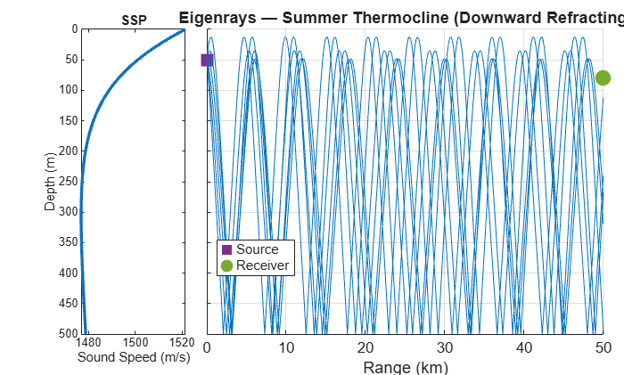

Now model the same geometry with constant sound speed.

bh_iso = bellhopModel;
bh_iso.SoundSpeed = 1500*ones(size(depth));
bh_iso.SoundSpeedDepth = depth;
bh_iso.RayElevationAngles = [-30 30];
bh_iso.RayTraceRangeLimit = 60000;
bh_iso.BottomBathymetryProfile = [0 500; 60000 500];
bh_iso.NumRays = 20;
propagationPaths(bh_iso, fc, srcPos, rxPos);
title("Eigenrays — Isospeed (1500 m/s)")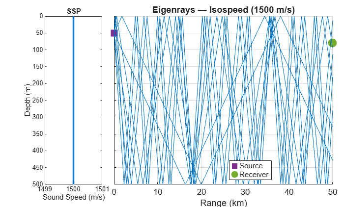

In the thermocline case, eigenrays curve downward and reach the receiver only via bottom-reflected paths, leaving a shadow zone in the upper water column. In the isospeed case, rays travel in straight lines with reflected paths distributing more uniformly between surface and bottom.

Model Range-Dependent Sound Speed

In many ocean environments, sound speed varies not only with depth but also with horizontal range. A well-known example is the Gulf Stream front off the US East Coast, where cold, nearly isothermal shelf water meets warm, stratified Gulf Stream water. The shelf profile is mildly upward-refracting (pressure effect dominates), while the Gulf Stream profile is strongly downward-refracting (thermocline dominates).

Define profiles at three range stations representing a Gulf Stream front. The source is on the continental shelf in nearly isothermal water (~12°C). The front is at 30 km, beyond which Gulf Stream water has a ~24°C surface and strong thermocline.

depth_rd = (0:10:500)';
temp_shelf = 12 - 1*(depth_rd/500);
c_shelf = underwaterSoundSpeed(temp_shelf, 34.5*ones(size(depth_rd)), depth_rd);
temp_front = 5 + 12*exp(-depth_rd/150);
c_front = underwaterSoundSpeed(temp_front, 35.2*ones(size(depth_rd)), depth_rd);
temp_gs = 5 + 19*exp(-depth_rd/120);
c_gs = underwaterSoundSpeed(temp_gs, 36*ones(size(depth_rd)), depth_rd);

Visualize the three profiles.

figure
plot(c_shelf, depth_rd, c_front, depth_rd, c_gs, depth_rd)
ax = gca;
ax.YDir = "reverse";
xlabel("Sound Speed (m/s)")
ylabel("Depth (m)")
legend("0 km (shelf water)", "30 km (front)", "60 km (Gulf Stream)")
title("Sound Speed Profiles — Gulf Stream Front")
grid on

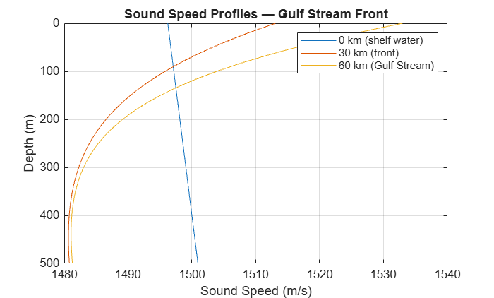
The shelf water has nearly uniform sound speed with a slight increase due to pressure. The Gulf Stream water shows a strong decrease near the surface where the thermocline dominates, with a ~50 m/s gradient over 500 m.

Compare the transmission loss of a range-independent SSP to a range-dependent profile. First, compute propagation using only the shelf profile as range-independent.

bh_shelf = bellhopModel;
bh_shelf.SoundSpeed = c_shelf;
bh_shelf.SoundSpeedDepth = depth_rd;
bh_shelf.RayElevationAngles = [-30 30];
bh_shelf.RayTraceRangeLimit = 60000;
bh_shelf.BottomBathymetryProfile = [0 500; 60000 500];
transmissionLoss(bh_shelf, fc, srcPos);
title("TL — Range-Independent (Shelf Water Only)")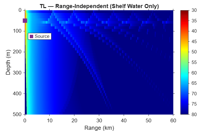

The nearly isothermal shelf water produces mild upward refraction. Rays curve toward the surface, distributing energy relatively uniformly with depth.

Now assemble the range-dependent model crossing the front.

bellhopModel supports range-dependent SSPs by accepting SoundSpeed as a matrix, where each column corresponds to a range station. Set SSPInterpolationMethod to "quadrilateral" so Bellhop interpolates the sound speed field between range stations. SoundSpeedRange must extend beyond RayTraceRangeLimit to produce a well-defined ray trace region for Bellhop.

bh_rd = bellhopModel;
bh_rd.SoundSpeed = [c_shelf, c_front, c_gs];
bh_rd.SoundSpeedDepth = depth_rd;
bh_rd.SoundSpeedRange = [0 30000 61000];
bh_rd.SSPInterpolationMethod = "quadrilateral";
bh_rd.RayElevationAngles = [-30 30];
bh_rd.RayTraceRangeLimit = 60000;
bh_rd.BottomBathymetryProfile = [0 500; 60000 500];
transmissionLoss(bh_rd, fc, srcPos);
title("TL — Gulf Stream Front (Shelf to Gulf Stream)")

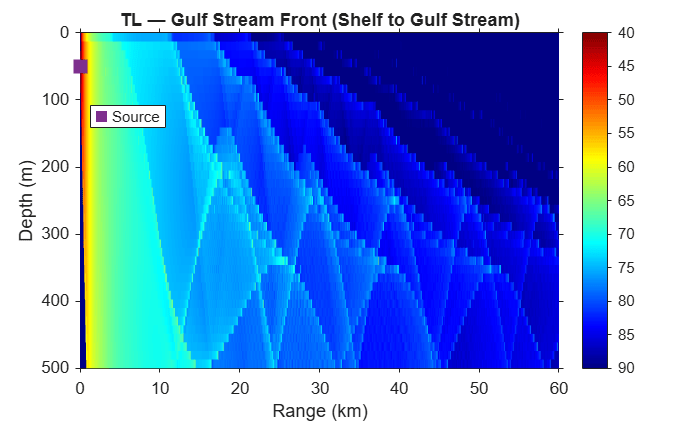
The range-dependent model shows how propagation differs across the front. In the shelf water (0–30 km), energy distributes relatively uniformly. Beyond the front, the strong Gulf Stream thermocline bends rays sharply downward, creating a surface shadow zone that does not appear in a range-independent model.

Generate Sea Surface Height from Wave Spectra

Wind-driven ocean waves create a rough air-water interface that scatters energy away from specular reflection paths. The seaSurfaceHeight function generates realistic 1-D sea surface realizations from wave energy spectra. The roughness depends on wind speed and fetch (distance over which wind blows).

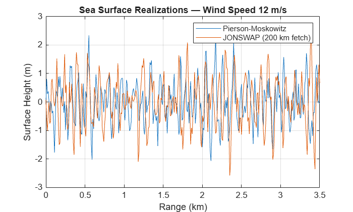
Generate a surface using the Pierson-Moskowitz (PM) spectrum for a fully developed sea at 12 m/s wind, a rough water condition characterized as sea state 5 by the World Meteorological Organization Sea State Code. Use 10 m resolution over a 3.5 km extent, a typical range for shallow-water sonar links.

rangeExtent = [0 3500];
resolution = 10;
eta_pm = seaSurfaceHeight(rangeExtent, resolution, SpectrumModel="pm", WindSpeed=12);

Generate a surface using the JONSWAP spectrum, which models fetch-limited wave growth and produces sharper spectral peaks.

eta_jw = seaSurfaceHeight(rangeExtent, resolution, SpectrumModel="jonswap", ...
    WindSpeed=12, Fetch=200000);

Compare the two surface realizations. JONSWAP waves are typically steeper and more regular than the fully developed PM spectrum.

figure
plot(eta_pm(:,1)/1000, eta_pm(:,2), eta_jw(:,1)/1000, eta_jw(:,2))
xlabel("Range (km)")
ylabel("Surface Height (m)")
legend("Pierson-Moskowitz", "JONSWAP (200 km fetch)")
title("Sea Surface Realizations — Wind Speed 12 m/s")
grid on

Examine Effect of Sea Surface on Multipath Reflections

At the ocean boundaries, reflections from the sea surface and bottom introduce multipath arrivals that interfere constructively or destructively at the receiver. In shallow water, acoustic paths bounce repeatedly between the surface and bottom. A rough sea surface disrupts these reflections by scattering energy away from the specular direction at each surface interaction. This disruption is most visible in shallow isospeed channels where rays travel in straight lines and undergo many surface bounces over short ranges.

Set up a shallow channel with 50 m depth, constant sound speed (1500 m/s), a source at 15 m depth, and a receiver at 3 km range and 25 m depth.

depthShallow = [0; 50];
cShallow = [1500; 1500];
srcShallow = [0; 0; 15];
rxShallow = [0; 3000; 25];
bh_flat = bellhopModel;
bh_flat.SoundSpeed = cShallow;
bh_flat.SoundSpeedDepth = depthShallow;
bh_flat.RayElevationAngles = [-10 10];
bh_flat.RayTraceRangeLimit = 3500;
bh_flat.NumRays = 10;
bh_flat.BottomBathymetryProfile = [0 50; 3500 50];

Compute eigenrays with a flat surface. In this isospeed channel, rays travel in straight lines and reflect specularly at both boundaries. The plot shows multiple bounce paths connecting source and receiver.

propagationPaths(bh_flat, fc, srcShallow, rxShallow);
title("Eigenrays — Flat Surface (50 m Shallow Channel)")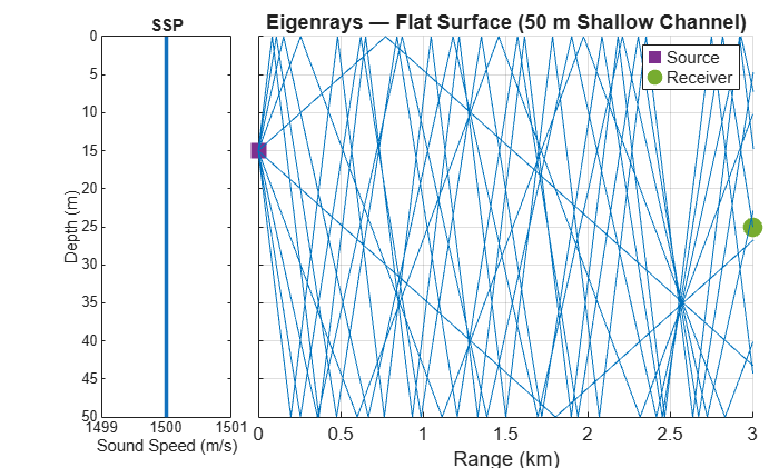

Now apply the rough sea surface and compute eigenrays through the same channel. The wave-induced surface undulations redirect reflected rays, preventing some high-order bounce paths from reaching the receiver.

bh_rough = bellhopModel;
bh_rough.SoundSpeed = cShallow;
bh_rough.SoundSpeedDepth = depthShallow;
bh_rough.RayElevationAngles = [-10 10];
bh_rough.RayTraceRangeLimit = 3500;
bh_rough.BottomBathymetryProfile = [0 50; 3500 50];
bh_rough.SurfaceAltimetryProfile = eta_pm;
bh_rough.NumRays = 10;
propagationPaths(bh_rough, fc, srcShallow, rxShallow);

Warning: SoundSpeed profile was automatically extended upward from depth 0 m to -2.351947 m using constant extrapolation to cover SurfaceAltimetryProfile.

title("Eigenrays — Rough Surface (Wind = 12 m/s)")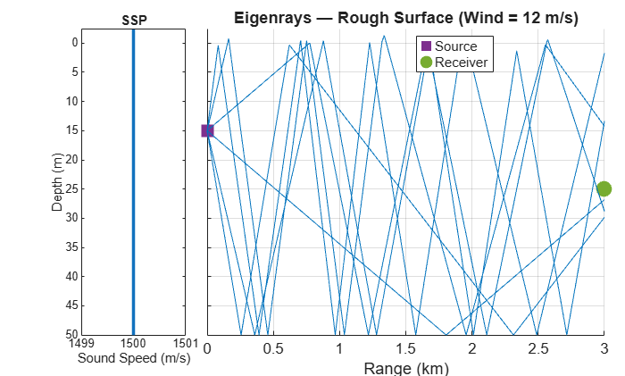

The SSP is defined from depth 0 m downward to the sea bottom. bellhopModel raises a warning when it extrapolates the SSP upward to compute the sound speed for wave crests.

Call propagationPaths again without plotting to retrieve the arrivals tables. Compare the number of arrivals.

arrivals_flat = propagationPaths(bh_flat, fc, srcShallow, rxShallow);
arrivals_rough = propagationPaths(bh_rough, fc, srcShallow, rxShallow);

Warning: SoundSpeed profile was automatically extended upward from depth 0 m to -2.351947 m using constant extrapolation to cover SurfaceAltimetryProfile.

disp("Flat surface:  " + height(arrivals_flat) + " arrivals")

Flat surface:  10 arrivals

disp("Rough surface: " + height(arrivals_rough) + " arrivals")

Rough surface: 6 arrivals

The rough surface scatters energy away from specular reflection paths, eliminating high-order bounces and reducing multipath complexity.

Model Littoral Channel with Sound Speed and Sloping Bathymetry

Bottom bathymetry modifies propagation by changing the angles and number of boundary interactions along different ray paths. In a littoral environment, the combined effect of a thermocline and sloping bathymetry determines which ray paths connect source and receiver. The thermocline bends rays downward while the deepening bottom allows steeper-angle reflections at longer ranges.

Define a summer thermocline for a 300 m coastal environment and a bottom that slopes from 120 m nearshore to 300 m at 30 km range.

depth_lit = (0:5:300)';
temp_lit = 22 - 16*(1 - exp(-depth_lit/60));
sal_lit = 34.5 + 0.5*(depth_lit/300);
c_lit = underwaterSoundSpeed(temp_lit, sal_lit, depth_lit);
bathymetry = [0 120; 10000 150; 20000 200; 30000 300];

Assemble the model and compute eigenrays from a source at 30 m depth to a receiver at 25 km range and 100 m depth.

bh_lit = bellhopModel;
bh_lit.SoundSpeed = c_lit;
bh_lit.SoundSpeedDepth = depth_lit;
bh_lit.BottomBathymetryProfile = bathymetry;
bh_lit.RayElevationAngles = [-45 45];
bh_lit.RayTraceRangeLimit = 30000;
srcPos_lit = [0; 0; 30];
rxPos_lit = [0; 25000; 100];
propagationPaths(bh_lit, 1000, srcPos_lit, rxPos_lit);
title("Eigenrays — Littoral Channel with Sloping Bottom")
hold on;
plot(bathymetry(:,1)/1000, bathymetry(:,2), 'k-', LineWidth=2,DisplayName="Bathymetry")
xlim([0 rxPos_lit(2)/1000])

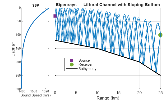
Retrieve the arrivals table. Each row is one eigenray with its path loss, delay, and count of boundary interactions. The downward-refracting profile combined with the sloping bottom limits the number of viable paths and increases bottom reflection counts at longer ranges.

arrivals_lit = propagationPaths(bh_lit, 1000, srcPos_lit, rxPos_lit)

arrivals_lit = 6×7 table
    PathLoss    PathDelay    PhaseShift    AngleOfDeparture    AngleOfArrival    NumSurfaceReflections    NumBottomReflections
    ________    _________    __________    ________________    ______________    _____________________    ____________________

     107.63       16.89       -73.035        0     7.9316       0    -4.3149               0                       12         
     117.69      16.894       -67.914        0    -9.2622       0    -5.5878               2                       12         
     119.75      16.897        164.59        0    -9.9953       0     6.1862               3                       12         
     128.41       16.92         59.61        0     10.595       0    -6.1664               3                       13         
     133.35      16.925        15.568        0     11.199       0     6.7989               5                       13         
     133.62      16.927        -15.13        0    -10.955       0    -6.4751               5                       13