Longitudinal Flying Quality Analysis for 3DOF Sky Hogg Longitudinal Airframe

This example shows how to use eigenvalue analysis to determine the longitudinal flying quality characteristics (long-period phugoid mode and short-period mode) for an airframe modeled in Simulink®.

Perform longitudinal flying quality analysis on a dynamic system (aircraft) using a linearized representation of the airframe's longitudinal dynamics for a trimmed flight condition. This example uses Simulink Control Design™ functions to generate a trimmed operating point and to derive a linear state-space model for that operating point directly from a nonlinear Simulink model. From that state space model, the example computes longitudinal flight modes and compares them against MIL-F-8785C Requirements.

To perform this analysis on an airframe of your own, use the Aerospace Blockset™ Flight Control Analysis Tools.

Create New Vehicle Model from Template

Create and open a new airframe model using the Aerospace Blockset 3DOF Longitudinal Airframe Template. When the project is loaded, an architecture model for an airframe and vehicle configuration data, environmental constants, and initial conditions are loaded to the model workspace.

shModel = 'SkyHoggFlyingQualities';
if ~bdIsLoaded(shModel)
    open_system(new_system(shModel,'FromTemplate',...
        'asb3DOFLongitudinalAirframeTemplate.sltx'));
end

Specify a Desired Trim Condition

Next, define a trim condition around which to linearize the model. Set position component Xe to non-steady state, and define non-zero initial conditions where applicable:

shOpSpec = operspec(shModel);
shOpSpec.States(1).SteadyState = 0; % Xe
shOpSpec.States(2).x = state.XD; % Ze
shOpSpec.States(3).x = state.Theta; % theta
shOpSpec.States(4).x = state.U; % u
shOpSpec.Inputs(1).Min = aircraft.Surfaces(1).Surfaces.MinimumValue; % elevator input min
shOpSpec.Inputs(1).Max = aircraft.Surfaces(1).Surfaces.MaximumValue; % elevator input max

Create an Operating Point

Use findop() to find an operating point that satisfies the trim constraints defined above. View the Operating Point Search Report that is printed by this function below. Note that the defined specifications are successfully met.

shOpTrim = trimAirframe(shModel, shOpSpec);

 Operating point search report:
---------------------------------

opreport = 
 Operating point search report for the Model SkyHoggFlyingQualities.
 (Time-Varying Components Evaluated at time t=0)

Operating point specifications were successfully met.
States: 
----------
    Min          x          Max        dxMin        dx         dxMax   
___________ ___________ ___________ ___________ ___________ ___________
                                                                       
(1.) Xe
   -Inf          0          Inf        -Inf      100.4727       Inf    
(2.) Ze
   -Inf        -2000        Inf          0      4.6793e-11       0     
(3.) theta
   -Inf      0.015416       Inf          0           0           0     
(4.) u
   -Inf      100.4607       Inf          0      7.9684e-13       0     
(5.) w
   -Inf       1.5488        Inf          0      3.4208e-11       0     
(6.) q
   -Inf          0          Inf          0      -4.4542e-12      0     

Inputs: 
----------
   Min         u         Max    
__________ __________ __________
                                
(1.) SkyHoggFlyingQualities/ElevatorCmd
   -20     4.2571e-06     20    

Outputs: 
----------
    Min          y          Max    
___________ ___________ ___________
                                   
(1.) SkyHoggFlyingQualities/LonStatesBus
   -Inf      0.015416       Inf    
   -Inf          0          Inf    
   -Inf     -4.4542e-12     Inf    
   -Inf          0          Inf    
   -Inf        -2000        Inf    
   -Inf      100.4607       Inf    
   -Inf       1.5488        Inf    
   -Inf     7.9684e-13      Inf    
   -Inf     3.4208e-11      Inf    

Linearize the Vehicle Model at a Trimmed Operating Point

Prior to linearizing the system, define a set of linear analysis points in the model. This example applies an input perturbation to the Elevator Command Input port. Output measurements are taken for states $$\theta$$ and $$q$$.

shLinSys = linearizeAirframe(shModel, shOpTrim)

shLinSys =
 
  A = 
                 u         w         q     theta
   u      -0.04429     0.114    -1.549    -9.809
   w       -0.1311    -4.164     100.5   -0.1512
   q      0.001931   -0.1253         0         0
   theta         0         0         1         0
 
  B = 
          ElevatorCmd
   u           0.1421
   w            17.86
   q           -9.267
   theta            0
 
  C = 
              u      w      q  theta
   q          0      0      1      0
   theta      0      0      0      1
 
  D = 
          ElevatorCmd
   q                0
   theta            0
 
Continuous-time state-space model.

View the linearization result as a continuous-time transfer function:

shLinSysTF = tf(shLinSys)

shLinSysTF =
 
  From input "ElevatorCmd" to output...
        -9.267 s^3 - 41.23 s^2 - 1.939 s + 8.368e-17
   q:  -----------------------------------------------
       s^4 + 4.208 s^3 + 12.79 s^2 + 0.5731 s + 0.2391
 
                    -9.267 s^2 - 41.23 s - 1.939
   theta:  -----------------------------------------------
           s^4 + 4.208 s^3 + 12.79 s^2 + 0.5731 s + 0.2391
 
Continuous-time transfer function.

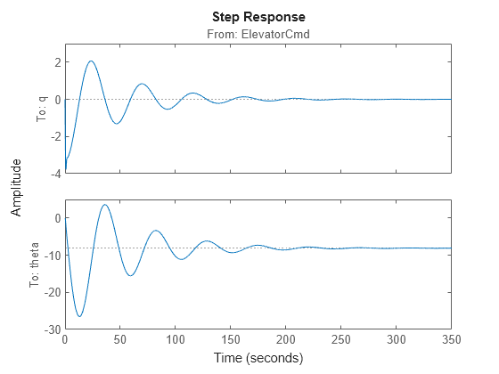
Examine the pitch response of the system to an elevator step input:

step(shLinSysTF)

Discussion of Longitudinal Characteristic Equation Roots and Their Connection to Dynamic Stability

To determine if the airframe is longitudinally, dynamically, stable at a particular operating point, examine the roots of the linear systems characteristic equation. In general, these roots are of the form:

$$\sigma =\eta \pm i\omega$$

where $$\eta$$ and $$\omega$$ are real numbers. These roots characterize the modes of the system longitudinal motion. The example uses these modes to determine stability:

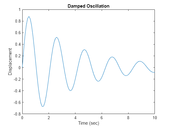
• If $$\eta$$ is negative and $$\omega$$ is nonzero, the motion is a periodic damped oscillation, as seen here.

eta = -0.25;
omega = 3;
t = 0:.1:10;
plot(t, exp(eta*t).*sin(omega*t));
ylabel('Displacement')
xlabel('Time (sec)')
title('Damped Oscillation')

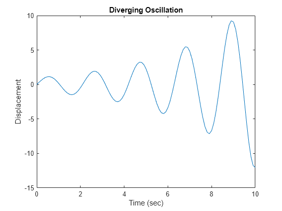
• If $$\eta$$ is positive and $$\omega$$ is nonzero, the motion is a periodic diverging oscillation.

eta = 0.25;
omega = 3;
plot(t, exp(eta*t).*sin(omega*t));
ylabel('Displacement')
xlabel('Time (sec)')
title('Diverging Oscillation')

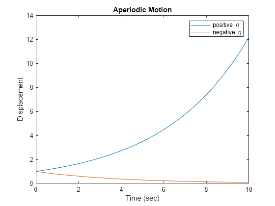
• If $$\omega$$ is zero, the motion is aperiodic. It diverges if $$\eta$$ is positive and converges if $$\eta$$ is negative.

plot(t, exp(.25*t))
hold on
plot(t, exp(-.25*t))
legend('positive \eta', 'negative \eta');
hold off
ylabel('Displacement')
xlabel('Time (sec)')
title('Aperiodic Motion')

Analyze the Longitudinal Dynamic Stability Characteristics of the Vehicle Model

Using the above criteria, it follows that any real root or real part of a root must be negative for the dynamic system to be stable. The roots of the computed state-space model are:

shRoots = eig(shLinSys)

shRoots = 4×1 complex

  -2.0844 + 2.8739i
  -2.0844 - 2.8739i
  -0.0196 + 0.1363i
  -0.0196 - 0.1363i

Visualize these roots using a Pole-Zero Plot. As discussed, for inherent stability all roots should have negative real components.

pzplot(shLinSysTF,'b')
grid on

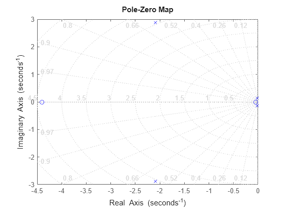
The roots are two pairs of complex conjugates. This is the most common for the longitudinal dynamics of stable aircraft. The complex conjugate pair with the higher frequency of oscillation (greater imaginary part) is the short-period mode. The complex conjugate pair with the lower frequency is the long-period or phugoid mode. Compute the damping ratio $$\zeta$$ and the undamped natural frequency $${\omega }_n$$ of each mode using the relationships:

$${\sigma }_{sp}={\zeta }_{sp}{\omega }_{n_{sp}}\pm i{\omega }_{n_{sp}}\sqrt{1-{\zeta }_{sp}^2}$$

and

$${\sigma }_{ph}={\zeta }_{ph}{\omega }_{n_{ph}}\pm i{\omega }_{n_{ph}}\sqrt{1-{\zeta }_{ph}^2}$$

Calculate Short-Period Mode Characteristics

Compute the damping ratio $$\zeta$$ and the undamped natural frequency $${\omega }_n$$ of the short-period mode using the relationship:

$${\sigma }_{sp}={\zeta }_{sp}{\omega }_{n_{sp}}\pm i{\omega }_{n_{sp}}\sqrt{1-{\zeta }_{sp}^2}$$

Short-Period Mode Damping Ratio

$${\zeta }_{sp}=\sqrt{1/(1+{\omega }_{sp}/{\eta }_{sp})}$$

$${\zeta }_{sp}=0.59$$

shZeta_sp = sqrt(1/(1+(imag(shRoots(1))/real(shRoots(1)))^2))

shZeta_sp = 
0.5871

Short-Period Mode Undamped Natural Frequency

$${\omega }_{n_{sp}}=-{\eta }_{sp}/{\zeta }_{sp}$$

$${\omega }_{n_{sp}}=3.55$$ rad/s

shOmega_n_sp = -real(shRoots(1))/shZeta_sp

shOmega_n_sp = 
3.5502

Time to Double the Short-Period Mode Amplitude

$$T_{2_{sp}}=ln(2)/(-{\zeta }_{sp}{\omega }_{sp})$$

$$T_{2_{sp}}=-0.33$$ sec

shT_2_sp = log(2)/(-shZeta_sp*shOmega_n_sp)

shT_2_sp = 
-0.3325

Note that the short-period mode damping ratio is positive, so the time-to-double the short-period mode amplitude is negative. This means that $$T_{2_{sp}}$$ actually represents the time-to-halve the short-period mode amplitude, or $$T_{1/2_{sp}}$$.

Calculate Phugoid Mode Characteristics

Compute the damping ratio $$\zeta$$ and the undamped natural frequency $${\omega }_n$$ of the phugoid mode using the relationship:

$${\sigma }_{ph}={\zeta }_{ph}{\omega }_{n_{ph}}\pm i{\omega }_{n_{ph}}\sqrt{1-{\zeta }_{ph}^2}$$

Phugoid Mode Damping Ratio

$${\zeta }_{ph}=\sqrt{1/(1+{\omega }_{ph}/{\eta }_{ph})}$$

$${\zeta }_{ph}=0.14$$

shZeta_ph = sqrt(1/(1+(imag(shRoots(3))/real(shRoots(3)))^2))

shZeta_ph = 
0.1423

Phugoid Mode Undamped Natural Frequency

$${\omega }_{n_{ph}}=-{\eta }_{ph}/{\zeta }_{ph}$$

$${\omega }_{n_{ph}}=0.14$$ rad/sec

shOmega_n_ph = -real(shRoots(3))/shZeta_ph

shOmega_n_ph = 
0.1377

Time to Double the Phugoid Mode Amplitude

$$T_{2_{ph}}=ln(2)/(-{\zeta }_{ph}{\omega }_{ph})$$

$$T_{2_{ph}}=-35.4$$ sec

shT_2_ph = log(2)/(-shZeta_ph*shOmega_n_ph)

shT_2_ph = 
-35.3727

Note that the phugoid mode damping ratio is positive, so the time-to-double the phugoid mode amplitude is negative. This means that $$T_{2_{ph}}$$ represents the time-to-halve the phugoid mode amplitude, or $$T_{1/2_{ph}}$$.

Compare Phugoid Response to Short-Period Response

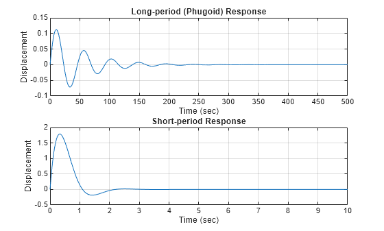
Observe that the short-period mode is much better damped than the phugoid mode.

$$f(t)=({\omega }_n/\sqrt{1-{\zeta }^2})e^{-\zeta \omega t}sin({\omega }_n\sqrt{1-{\zeta }^2}t)$$

Note the difference in time scales.

figure;

subplot(2,1,1)
t = 0:.1:500;
plot(t, shOmega_n_ph/sqrt(1-shZeta_ph^2).*exp(-shZeta_ph*shOmega_n_ph*t).*sin(shOmega_n_ph*sqrt(1-shZeta_ph^2)*t))
ylabel('Displacement')
xlabel('Time (sec)')
title('Long-period (Phugoid) Response')
grid on

subplot(2,1,2)
t = 0:.025:10;
plot(t, shOmega_n_sp/sqrt(1-shZeta_sp^2).*exp(-shZeta_sp*shOmega_n_sp*t).*sin(shOmega_n_sp*sqrt(1-shZeta_sp^2)*t))
ylabel('Displacement')
xlabel('Time (sec)')
title('Short-period Response')
grid on

The above analysis can also be quickly performed using computeLongitudinalFlyingQualities(shModel, shLinSys).

longFlyingQual = computeLongitudinalFlyingQualities(shModel, shLinSys)

longFlyingQual = struct with fields:
        PhugoidMode: [1x1 struct]
    ShortPeriodMode: [1x1 struct]

phugoidModeStruct = longFlyingQual.PhugoidMode

phugoidModeStruct = struct with fields:
                    root: [2x1 double]
         oscillatoryMode: 'Phugoid (Long-Period Mode)'
                    zeta: 0.1423
                      wn: 0.1377
                      T2: -35.3727
                      Tc: []
                response: 'converging oscillatory motion'
             description: 'complex conjugate pair with negative real components'
       RequirementSource: "MIL-F-8785C"
         RequirementName: "Phugoid Stability"
                      ID: "3.2.1.2"
      FlyingQualityLevel: "1"
             FlightPhase: "B"
           AircraftClass: ["I"    "II"    "III"    "IV"]
                Verified: 1
    MILF8785CRequirement: 'Satisfies MIL-F-8785C Level 1 Criteria (zeta_ph >= 0.04)'

MIL-F-8785C Longitudinal Flying Quality Requirements

Flying quality requirements are presented for three levels of flying qualities. These flying quality levels, in decreasing order of desirability, are:

• Level 1: Flying qualities clearly adequate to accomplish mission flight phase. Corresponds with Cooper-Harper Scale values 1-3.5.

• Level 2: Flying qualities adequate to accomplish mission flight phase with some increase in pilot workload required or degradation in mission effectiveness. Corresponds with Cooper-Harper Scale values 3.5-6.5.

• Level 3: Flying qualities adequate for airplane to be safely controlled, but excessive pilot workload is required or mission effectiveness is inadequate. Corresponds with Cooper-Harper Scale values 6.5-9+.

Note that airplanes must be designed to satisfy Level 1 requirements with all systems in their normal operating state.

Phugoid Mode Damping Requirements

Per MIL-F-8785C, the long-period airspeed oscillations (phugoid) which occur when an airplane seeks a stabilized airspeed following a disturbance must meet the following minimum requirements:

Level 1: $${\zeta }_{ph}>=0.04$$

Level 2: $${\zeta }_{ph}>=0.0$$

Level 3: $$T_{2_{ph}}>=55$$ sec

where $${\zeta }_{ph}$$ is the Phugoid Damping Ratio and $$T_{2_{ph}}$$ is the time-to-double the phugoid amplitude.

With $${\zeta }_{ph}=0.14$$, it is clear that the phugoid mode for this aircraft meets the Level 1 criteria of the MIL-F-8785C standard.

Short-Period Mode Damping Limits

MIL-F-8785C outlines recommended upper and lower limits for the short-period damping ratio. If damping is too low, short-period response can produce troublesome oscillation, and if damping is too high, response to control inputs can be sluggish. The following requirements are for Flight Phase B (all airplane classes) as defined in MIL-F-8785C (non-terminal flight phases that are normally accomplished using gradual maneuvers - climb, cruise, loiter, descent, etc.):

Level 1: $$0.30<{\zeta }_{sp}<2.00$$

Level 2: $$0.20<{\zeta }_{sp}<2.00$$

Level 3: $$0.15<{\zeta }_{sp}$$

where $${\zeta }_{sp}$$ is the short-period damping ratio.

With $${\zeta }_{sp}=0.59$$, the short-period mode for this aircraft meets the Level 1 criteria of the MIL-F-8785C standard.

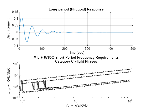
Short Period Category C Requirements Plot

The reference MIL-F-8785C short-period category C requirements can be plotted using shortPeriodCategoryCPlot

shortPeriodCategoryCPlot([])

References

[1] Moorehouse, David J., Woodcock, Robert J., "Background Information and User Guide For MIL-F-8785C, Military Specification - Flying Qualities of Piloted Airplanes", AFWAL-TR-81-3109, July 1982.

[2] Roskam, J., "Airplane Flight Dynamics and Automatic Flight Controls (Part 1)", DAR Corporation, 2003.

[3] McCormick, B.W. "Aerodynamics, Aeronautics, and Flight Mechanics" 2rd Ed., John Wiley & Sons Inc., 1995.