Symbolic Math Toolbox による解析プロット

ライブスクリプトを開く

Symbolic Math Toolbox™ は、数値データを明示的に生成することなく数式の解析プロットを提供します。これらのプロットは、2 次元または 3 次元のラインプロット、曲線プロット、等高線図、表面プロットまたはメッシュプロットになります。

これらの例では、シンボリック関数、式、および方程式を入力として受け入れる以下のグラフィックス関数について扱います。

fplot
fimplicit
fcontour
fplot3
fsurf
fmesh
fimplicit3

`fplot` を使用した陽関数 $y = f (x)$ のプロット

関数 $\sin (\exp (x))$ をプロットします。

syms x
fplot(sin(exp(x)))

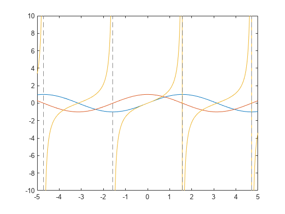
Figure contains an axes object. The axes object contains an object of type functionline.

三角関数 $\sin (x)$ 、 $\cos (x)$ 、および $\tan (x)$ を同時にプロットします。

fplot([sin(x),cos(x),tan(x)])

Figure contains an axes object. The axes object contains 3 objects of type functionline.

$y = f (x, a)$ によって定義された関数の、さまざまな $a$ の値によるプロット

関数 $\sin (\exp (x / a))$ を、 $a = 1, 2$ および $4$ についてプロットします。

syms x a
expr = sin(exp(x/a));
fplot(subs(expr,a,[1,2,4]))
legend show

Figure contains an axes object. The axes object contains 3 objects of type functionline.

関数の微分と積分のプロット

関数 $f (x) = x (1 + x) + 2$ 、その微分 $d f (x) / d x$ 、およびその積分 $\int f (x) d x$ をプロットします。

syms f(x)
f(x) = x*(1 + x) + 2

f(x) =  $x (x + 1) + 2$

f_diff = diff(f(x),x)

f_diff =  $2 x + 1$

f_int = int(f(x),x)

f_int = 
 $\frac{x (2 x^{2} + 3 x + 12)}{6}$

fplot([f,f_diff,f_int])
legend({'$f(x)$','$df(x)/dx$','$\int f(x)dx$'},'Interpreter','latex','FontSize',12)

$Figure contains an axes object. The axes object contains 3 objects of type functionline. These objects represent $f(x)$, $df(x)/dx$, $\int f(x)dx$.$

$a$ を横軸とする関数 $y = g (x_{0}, a)$ のプロット

微分方程式 $d g (x, a) / d x = 0$ を解いて、関数 $g (x, a)$ を最小化する $x_{0}$ を求めます。

syms g(x,a);
assume(a>0);
g(x,a) = a*x*(a + x) + 2*sqrt(a)

g(x, a) =  $2 \sqrt{a} + a x (a + x)$

x0 = solve(diff(g,x),x)

x0 = 
 $- \frac{a}{2}$

0 から 5 までの $a$ について $g (x_{0}, a)$ の最小値をプロットします。

fplot(g(x0,a),[0 5])
xlabel('a')
title('Minimum Value of $g(x_0,a)$ Depending on $a$','interpreter','latex')

Figure contains an axes object. The axes object with title Minimum Value of g leftParenthesis x indexOf 0 baseline , a rightParenthesis Depending on a, xlabel a contains an object of type functionline.

`fimplicit` を使用した陰関数 $f (x, y) = c$ のプロット

$x^{2} + y^{2} = r^{2}$ によって定義された円を、1 から 10 までの整数の半径 $r$ でプロットします。

syms x y
r = 1:10;
fimplicit(x^2 + y^2 == r.^2,[-10 10])
axis square;

Figure contains an axes object. The axes object contains 10 objects of type implicitfunctionline.

`fcontour` を使用した関数 $f (x, y)$ の等高線のプロット

関数 $f (x, y) = x^{3} - 4 x - y^{2}$ の等高線を、–6 から 6 までの等高線レベルについてプロットします。

syms x y f(x,y)
f(x,y) = x^3 - 4*x - y^2;
fcontour(f,[-3 3 -4 4],'LevelList',-6:6);
colorbar
title 'Contour of Some Elliptic Curves'

Figure contains an axes object. The axes object with title Contour of Some Elliptic Curves contains an object of type functioncontour.

スプライン内挿を使用した解析関数とその近似のプロット

解析関数 $f (x) = x \exp (- x) \sin (5 x) - 2$ をプロットします。

syms f(x)
f(x) = x*exp(-x)*sin(5*x) -2;
fplot(f,[0,3])

解析関数からいくつかのデータ点を作成します。

xs = 0:1/3:3;
ys = double(subs(f,xs));

データ点と、解析関数を近似するスプライン内挿をプロットします。

hold on
plot(xs,ys,'*k','DisplayName','Data Points')
fplot(@(x) spline(xs,ys,x),[0 3],'DisplayName','Spline interpolant')
grid on
legend show
hold off

Figure contains an axes object. The axes object contains 3 objects of type functionline, line. One or more of the lines displays its values using only markers These objects represent Data Points, Spline interpolant.

関数のテイラー近似のプロット

$\cos (x)$ の、最大 5 階および 7 階までの $x = 0$ 付近のテイラー展開を求めます。

syms x
t5 = taylor(cos(x),x,'Order',5)

t5 = 
 $\frac{x^{4}}{24} - \frac{x^{2}}{2} + 1$

t7 = taylor(cos(x),x,'Order',7)

t7 = 
 $- \frac{x^{6}}{720} + \frac{x^{4}}{24} - \frac{x^{2}}{2} + 1$

$\cos (x)$ とそのテイラー近似をプロットします。

fplot(cos(x))
hold on;
fplot([t5 t7],'--')
axis([-4 4 -1.5 1.5])
title('Taylor Series Approximations of cos(x) up to 5th and 7th Order')
legend show
hold off;

Figure contains an axes object. The axes object with title Taylor Series Approximations of cos(x) up to 5th and 7th Order contains 3 objects of type functionline.

矩形波のフーリエ級数近似のプロット

周期 $2 π$ 、振幅 $π / 4$ の矩形波は、次のフーリエ級数展開で近似できます。

$\sin (t) + \frac{1}{3} \sin (3 t) + \frac{1}{5} \sin (5 t) + . . . .$

周期 $2 π$ 、振幅 $π / 4$ の矩形波をプロットします。

syms t y(t)
y(t) = piecewise(0 < mod(t,2*pi) <= pi, pi/4, pi < mod(t,2*pi) <= 2*pi, -pi/4);
fplot(y)

この矩形波のフーリエ級数近似をプロットします。

hold on;
n = 6;
yFourier = cumsum(sin((1:2:2*n-1)*t)./(1:2:2*n-1));
fplot(yFourier,'LineWidth',1)
hold off

Figure contains an axes object. The axes object contains 7 objects of type functionline.

フーリエ級数近似はジャンプ不連続点でオーバーシュートし、近似に項が追加されても "リンギング" は解消しません。この動作は、ギブス現象としても知られています。

`fplot3` を使用したパラメトリック曲線 $(x (t), y (t), z (t))$ のプロット

$(\sin (t), \cos (t), t / 4)$ によって定義されるらせんを、–10 から 10 までの $t$ についてプロットします。

syms t
fplot3(sin(t),cos(t),t/4,[-10 10],'LineWidth',2)
view([-45 45])

Figure contains an axes object. The axes object contains an object of type parameterizedfunctionline.

`fsurf` を使用した $z = f (x, y)$ によって定義される表面のプロット

$\log (x) + \exp (y)$ で定義される表面をプロットします。fsurf を使用した解析プロットでは、(数値データを生成することなく) 曲面と $x = 0$ 付近の漸近領域を表示します。

syms x y
fsurf(log(x) + exp(y),[0 2 -1 3])
xlabel('x')

Figure contains an axes object. The axes object with xlabel x contains an object of type functionsurface.

`fsurf` を使用した多変数表面 $(x (u, v), y (u, v), z (u, v))$ のプロット

以下によって定義される多変数表面をプロットします。

$x (u, v) = u$

$y (u, v) = f (u) \sin (v)$

$z (u, v) = f (u) \cos (v)$

ここで、 $f (u) = \exp (- u^{2} / 3) \sin (u) + 3 / 2$ です。

$u$ のプロット区間を –5 から 5 まで、 $v$ のプロット区間を 0 から 2 $π$ までに設定します。

syms f(u) x(u,v) y(u,v) z(u,v)
f(u) = sin(u)*exp(-u^2/3)+1.5;
x(u,v) = u;
y(u,v) = f(u)*sin(v);
z(u,v) = f(u)*cos(v);
fsurf(x,y,z,[-5 5 0 2*pi])

Figure contains an axes object. The axes object contains an object of type parameterizedfunctionsurface.

`fmesh` を使用した多変数表面 $(x (s, t), y (s, t), z (s, t))$ のプロット

以下によって定義される多変数表面をプロットします。

$x = r \cos (s) \sin (t)$

$y = r \sin (s) \sin (t)$

$z = r \cos (t)$

ここで、 $r = 8 + \sin (7 s + 5 t)$ です。fmesh を使用して、プロットされた表面をメッシュとして表示します。 $s$ のプロット区間を 0 から 2 $π$ まで、 $t$ のプロット区間を 0 から $π$ までに設定します。

syms s t
r = 8 + sin(7*s + 5*t);
x = r*cos(s)*sin(t);
y = r*sin(s)*sin(t);
z = r*cos(t);
fmesh(x,y,z,[0 2*pi 0 pi],'Linewidth',2)
axis equal

Figure contains an axes object. The axes object contains an object of type parameterizedfunctionsurface.

`fimplicit3` を使用した陰関数表面 $f (x, y, z) = c$ のプロット

陰関数表面 $1 / x^{2} - 1 / y^{2} + 1 / z^{2} = 0$ をプロットします。

syms x y z
f = 1/x^2 - 1/y^2 + 1/z^2;
fimplicit3(f)

Figure contains an axes object. The axes object contains an object of type implicitfunctionsurface.

表面の等高線と勾配のプロット

fsurf を使用して表面 $\sin (x) + \sin (y) - (x^{2} + y^{2}) / 20$ をプロットします。'ShowContours' を 'on' に設定して、同じグラフに等高線を表示できます。

syms x y
f = sin(x)+sin(y)-(x^2+y^2)/20

f = 
 $\sin (x) + \sin (y) - \frac{x^{2}}{20} - \frac{y^{2}}{20}$

fsurf(f,'ShowContours','on')
view(-19,56)

Figure contains an axes object. The axes object contains an object of type functionsurface.

次に、より細かい等高線の間隔で別のグラフに等高線をプロットします。

fcontour(f,[-5 5 -5 5],'LevelStep',0.1,'Fill','on')
colorbar

表面の勾配を求めます。meshgrid を使用して 2 次元グリッドを作成してグリッド座標を代入し、勾配を数値的に評価します。quiver を使用して勾配を表示します。

hold on
Fgrad = gradient(f,[x,y])

Fgrad = 
 $(\begin{array}{c} \cos (x) - \frac{x}{10} \\ \cos (y) - \frac{y}{10} \end{array})$

[xgrid,ygrid] = meshgrid(-5:5,-5:5);
Fx = subs(Fgrad(1),{x,y},{xgrid,ygrid});
Fy = subs(Fgrad(2),{x,y},{xgrid,ygrid});
quiver(xgrid,ygrid,Fx,Fy,'k')
hold off

Figure contains an axes object. The axes object contains 2 objects of type functioncontour, quiver.

参考

関数

fplot | fimplicit | fcontour | fplot3 | fsurf | fmesh | fimplicit3

Symbolic Math Toolbox による解析プロット

fplot を使用した陽関数 y=f(x) のプロット

y=f(x,a) によって定義された関数の、さまざまな a の値によるプロット

関数の微分と積分のプロット

a を横軸とする関数 y=g(x0,a) のプロット

fimplicit を使用した陰関数 f(x,y)=c のプロット

fcontour を使用した関数 f(x,y) の等高線のプロット