このページの内容は最新ではありません。最新版の英語を参照するには、ここをクリックします。
IIR フィルターの浮動小数点から固定小数点への変換
この例では、固定小数点コンバーター アプリを使用して IIR フィルターを浮動小数点から固定小数点の実装に変換する方法を説明します。二次型 (または "双二次") の構造は、伝達関数を直接実装する構造よりも、固定小数点演算を使用する場合にうまく機能します。ここでは、"浮動から固定" の変換を成功させるための最も確実な方法を説明します。この方法は、以下の手順で構成されています。
2 次セクション (SOS) 構造、つまり
dsp.BiquadFilterを選択フィルターの各ノードのダイナミック レンジ解析を実行。つまり、シミュレーションの最小値とシミュレーションの最大値のインストルメンテーションによるテスト ベンチ アプローチを使用
代替方法である双二次スケーリング実装と比較し、'
fvtool' およびpectrumAnalyzerを使用して解析および検証して、異なる選択に起因する量子化の影響を表示
はじめに
IIR フィルターを効率的に実装する方法として、2 次セクション (SOS) 双二次フィルター構造を使用する方法があります。たとえば、システムから高周波数のトーン信号である干渉源を除去する必要があると仮定します。これを実行する方法の 1 つは、ローパス フィルター設計を使用することです。
ローパス楕円フィルターの設計
この例では、最小次数のローパス楕円直接型 I 設計を使用します。フィルターの設計仕様は、以下のとおりです。
通過帯域周波数エッジ:
阻止帯域周波数エッジ:
通過帯域リップル:
阻止帯域の減衰量:
フィルターの可視化ツールを使用して、すべての 2 次セクションの累積フィルター応答を可視化します。
biquad = design(fdesign.lowpass('Fp,Fst,Ap,Ast',0.4,0.45,0.5,80), ...
    'ellip',FilterStructure='df1sos', SystemObject=true, UseLegacyBiquadFilter=true);
fvt = fvtool(biquad, Legend='on');
fvt.SosviewSettings.View = 'Cumulative';

浮動小数点と固定小数点の比較に用いるフィルター係数 (SOS、B、A) の取得
SOS フィルター係数値は (double または 16 ビット固定小数点値のどちらの場合にも) ほぼ同じフィルター応答を導くことに注意してください。
sosMatrix = biquad.SOSMatrix;
sclValues = biquad.ScaleValues;
fvt_comp = fvtool(sosMatrix,fi(sosMatrix,1,16));
legend(fvt_comp,'Floating-point (double) SOS','Fixed-point (16-bit) SOS');

b = repmat(sclValues(1:(end-1)),1,3) .* sosMatrix(:,(1:3));
a = sosMatrix(:,(5:6));
num = b'; % matrix of scaled numerator sections
den = a'; % matrix of denominator sections
close(fvt);      % clean up
close(fvt_comp); % clean up
既定の浮動小数点演算
フィルターを通して何らかのデータをストリーミングし、入出力応答を表示してフィルターの動作を検証します。まず、付加的な高周波数トーンの干渉源をともなう (浮動小数点の) 疑似ランダム ノイズ信号 (300 Hz でサンプリングされた信号) のフィルター処理を試行し、トーンが除去されるかを確認します。これは後でテスト ベンチの基準信号として使用します。
Wo           = 75/(300/2); % 75 Hz tone; system running at 300 Hz
inp_len      = 4000;       % Number of input samples (signal length)
inp_itf      = 0.5 .* sin((pi*Wo) .* (0:(inp_len-1))'); % tone interferer
scope = spectrumAnalyzer(SampleRate=300, ...
    PlotAsTwoSidedSpectrum=false, ...
    ShowLegend=true, YLimits=[-85 25], ...
    Title='Floating-Point Input Signal and Filter Output Signal', ...
    ChannelNames={'Floating-Point Input','Filter Output'});
rng(12345); % seed the rng for repeatable results
biquadLPFiltFloat = dsp.BiquadFilter(SOSMatrixSource='Input port', ...
    ScaleValuesInputPort=false);
for k = 1:10
    inp_sig = rand(inp_len,1) - 0.5; % random values in range (-0.5, 0.5)
    input = inp_sig + inp_itf; % combined input signal, range (-1.0, 1.0)
    out_1 = biquadLPFiltFloat(input,num,den); % filter
    scope([input,out_1]) % visualize input and filtered output
end

clear scope biquadLPFiltFloat; % clean up
既定の固定小数点演算
今度はオブジェクトの既定の設定を使用して、フィルターに何らかの固定小数点データを通します。固定小数点の既定の動作は無効な結果の原因となることに注意してください。
scope = spectrumAnalyzer(SampleRate=300, ...
    PlotAsTwoSidedSpectrum=false, ...
    ShowLegend=true, YLimits=[-85 25], ...
    Title='Fixed-Point Input Signal and Filter Output Signal', ...
    ChannelNames={'Fixed-Point Input','Default (Incorrect) Fixed-Point Output'});
rng(12345); % seed the rng for repeatable results
bqLPFiltFixpt = dsp.BiquadFilter(SOSMatrixSource='Input port', ...
    ScaleValuesInputPort=false);
for k = 1:10
    inp_sig = rand(inp_len,1) - 0.5;  % random values in range (-0.5, 0.5)
    inputFi = fi(inp_sig + inp_itf, 1, 16, 15); % signal range (-1.0, 1.0)
    out_2 = bqLPFiltFixpt(inputFi,fi(num,1,16),fi(den,1,16));
    scope([inputFi,out_2]) % visualize
end

clear scope bqLPFiltFixpt; % clean up
浮動小数点双二次 IIR フィルター関数の固定小数点への変換
オブジェクトの既定の固定小数点設定の代わりに、固定小数点コンバーター アプリを使用してオブジェクトを固定小数点に変換します。この方法によって、フィルターの実装内における個々の固定小数点型の可視性および制御性が向上し、固定小数点演算がより正確になります。
まず、固定小数点コンバーター アプリを使用する準備として、すべてのフィルターのデータ型の選択を "Custom" に設定し、変換する関数を作成します。
type myIIRLowpassBiquad;function output = myIIRLowpassBiquad(inp,num,den)
%myIIRNotchBiquad Biquad lowpass filter implementation
% Used as part of a MATLAB Fixed Point Converter App example.
% Copyright 2016-2021 The MathWorks, Inc.
persistent bqLPFilter;
if isempty(bqLPFilter)
bqLPFilter = dsp.BiquadFilter( ...
'SOSMatrixSource','Input port', ...
'ScaleValuesInputPort', false, ...
'SectionInputDataType', 'Custom', ...
'SectionOutputDataType', 'Custom', ...
'NumeratorProductDataType', 'Custom', ...
'DenominatorProductDataType', 'Custom', ...
'NumeratorAccumulatorDataType', 'Custom', ...
'DenominatorAccumulatorDataType', 'Custom', ...
'StateDataType', 'Custom', ...
'OutputDataType', 'Custom');
end
output = bqLPFilter(inp, num, den);
end
テスト ベンチ スクリプトの作成
データ型で制御されるすべての信号パスについて、シミュレーションの最小値とシミュレーションの最大値をシミュレートし、インストルメント化したこれらの値を収集するテスト ベンチを作成します。これにより、その後ツールでオートスケールされた固定小数点設定を推奨できるようになります。上記のコードの一部をテスト ベンチ スクリプトとして使用し、浮動小数点の入力から始めてテスト ベンチを検証した後、最小および最大データをシミュレートして収集します。その後、固定小数点コンバーター アプリを使用し、浮動小数関数の実装を固定小数点関数の実装に変換します。
type myIIRLowpassBiquad_tb.m;%% Test Bench for myIIRLowpassBiquad.m
% Copyright 2016-2021 The MathWorks, Inc.
%% Pre-designed filter (coefficients stored in MAT file):
% f = design(fdesign.lowpass('Fp,Fst,Ap,Ast',0.4,0.45,0.5,80), ...
% 'ellip', FilterStructure='df1sos',SystemObject=true);
% sosMatrix = f.SOSMatrix;
% sclValues = f.ScaleValues;
% b = repmat(sclValues(1:(end-1)),1,3) .* sosMatrix(:,(1:3));
% a = sosMatrix(:,(5:6));
% num = b';
% den = a';
% save('myIIRLowpassBiquadDesign.mat', 'b', 'a', 'num', 'den');
load('myIIRLowpassBiquadDesign.mat');
%% Interference signal, using values in range (-0.5, 0.5)
Wo = 75/(300/2); % 75 Hz tone; system running at 300 Hz
inp_len = 4000; sinTvec = (0:(inp_len-1))';
inp_itf = 0.5 .* sin((pi*Wo) .* sinTvec);
%% Filtering and visualization
% Filter an input signal, including an interference
% tone, to see if the tone is successfully removed.
rng(12345); % seed the rng for repeatable results
scope = spectrumAnalyzer(SampleRate=300,...
PlotAsTwoSidedSpectrum=false,ShowLegend=true,YLimits=[-125 25],...
Title='Input Signal and Filter Output Signal', ...
ChannelNames={'Input', 'Filter Output'});
for k = 1:10
inp_sig = rand(inp_len,1) - 0.5; % random values in range (-0.5, 0.5)
inp = inp_sig + inp_itf;
out_1 = myIIRLowpassBiquad(inp,num,den); % filter
scope([inp,out_1]); % visualize
end
固定小数点コンバーター アプリを使用した固定小数点への変換
固定小数点コンバーター アプリを起動します。このツールを起動するには、MATLAB® の [アプリ] メニューと 'fixedPointConverter' コマンドとの 2 つの方法があります。
変換する関数を [エントリポイント関数] フィールドに入力します。

テスト ベンチのスクリプト名を入力して入力を定義します。

テスト ベンチをシミュレートして範囲を収集するには [解析] をクリックします。
収集された [シミュレーションの最小値]、[シミュレーションの最大値] および [推奨された型] の値を観察します。

必要に応じて [推奨された型] フィールドを調整します。
[変換] をクリックして固定小数点コードを生成してレポートを表示します。

結果として得られる固定小数点の MATLAB 実装
生成された固定小数点関数の実装は次のようになります。
type myIIRLowpassBiquad_fixpt;%%%%%%%%%%%%%%%%%%%%%%%%%%%%%%%%%%%%%%%%%%%%%%%%%%%%%%%%%%%%%%%%%%%%%%%%%%%%
% %
% Generated by MATLAB 9.3 and Fixed-Point Designer 6.0 %
% %
%%%%%%%%%%%%%%%%%%%%%%%%%%%%%%%%%%%%%%%%%%%%%%%%%%%%%%%%%%%%%%%%%%%%%%%%%%%%
%#codegen
function output = myIIRLowpassBiquad_fixpt(inp,num,den)
%myIIRNotchBiquad Biquad lowpass filter implementation
% Used as part of a MATLAB Fixed Point Converter App example.
% Copyright 2016 The MathWorks, Inc.
fm = get_fimath();
persistent bqLPFilter;
if isempty(bqLPFilter)
bqLPFilter = dsp.BiquadFilter( ...
'SOSMatrixSource', 'Input port', ...
'ScaleValuesInputPort', false, ...
'SectionInputDataType', 'Custom', ...
'SectionOutputDataType', 'Custom', ...
'NumeratorProductDataType', 'Custom', ...
'DenominatorProductDataType', 'Custom', ...
'NumeratorAccumulatorDataType', 'Custom', ...
'DenominatorAccumulatorDataType', 'Custom', ...
'StateDataType', 'Custom', ...
'OutputDataType', 'Custom' , ...
'CustomSectionInputDataType', numerictype([], 16, 8), ...
'CustomSectionOutputDataType', numerictype([], 16, 8), ...
'CustomNumeratorProductDataType', numerictype([], 32, 26), ...
'CustomDenominatorProductDataType', numerictype([], 32, 23), ...
'CustomNumeratorAccumulatorDataType', numerictype([], 32, 24), ...
'CustomDenominatorAccumulatorDataType', numerictype([], 32, 23), ...
'CustomStateDataType', numerictype([], 16, 8), ...
'CustomOutputDataType', numerictype([], 16, 15));
end
output = fi(bqLPFilter(inp, num, den), 1, 16, 15, fm);
end
function fm = get_fimath()
fm = fimath('RoundingMethod', 'Floor',...
'OverflowAction', 'Wrap',...
'ProductMode','FullPrecision',...
'MaxProductWordLength', 128,...
'SumMode','FullPrecision',...
'MaxSumWordLength', 128);
end
コマンド ライン API を使用した固定小数点変換の自動化
別の方法として、コマンド ライン API を使用して固定小数点変換を自動化することもできます。
type myIIRLowpassF2F_prj_script;%%%%%%%%%%%%%%%%%%%%%%%%%%%%%%%%%%%%%%%%%%%%%%%%%%%%%%%%%%%%%%%%%%%%%%%%%%%%%%%%
% Script generated from project 'myIIRLowpassBiquad.prj' on 16-Oct-2014.
%%%%%%%%%%%%%%%%%%%%%%%%%%%%%%%%%%%%%%%%%%%%%%%%%%%%%%%%%%%%%%%%%%%%%%%%%%%%%%%%
%%%%%%%%%%%%%%%%%%%%%%%%%%%%%%%%%%%%%%%%%%%%%%%%%%%%%%%%%%%%%%%%%%%%%%%%%%%%%%%%
% Create configuration object of class 'coder.FixPtConfig'.
%%%%%%%%%%%%%%%%%%%%%%%%%%%%%%%%%%%%%%%%%%%%%%%%%%%%%%%%%%%%%%%%%%%%%%%%%%%%%%%%
cfg = coder.config('fixpt');
cfg.TestBenchName = { sprintf('S:\\Work\\15aFeatureExamples\\biquad_notch_f2f\\myIIRLowpassBiquad_tb.m') };
cfg.DefaultWordLength = 16;
cfg.LogIOForComparisonPlotting = true;
cfg.TestNumerics = true;
%%%%%%%%%%%%%%%%%%%%%%%%%%%%%%%%%%%%%%%%%%%%%%%%%%%%%%%%%%%%%%%%%%%%%%%%%%%%%%%%
% Define argument types for entry-point 'myIIRLowpassBiquad'.
%%%%%%%%%%%%%%%%%%%%%%%%%%%%%%%%%%%%%%%%%%%%%%%%%%%%%%%%%%%%%%%%%%%%%%%%%%%%%%%%
ARGS = cell(1,1);
ARGS{1} = cell(3,1);
ARGS{1}{1} = coder.typeof(0,[4000 1]);
ARGS{1}{2} = coder.typeof(0,[3 5]);
ARGS{1}{3} = coder.typeof(0,[2 5]);
%%%%%%%%%%%%%%%%%%%%%%%%%%%%%%%%%%%%%%%%%%%%%%%%%%%%%%%%%%%%%%%%%%%%%%%%%%%%%%%%
% Invoke MATLAB Coder.
%%%%%%%%%%%%%%%%%%%%%%%%%%%%%%%%%%%%%%%%%%%%%%%%%%%%%%%%%%%%%%%%%%%%%%%%%%%%%%%%
codegen -float2fixed cfg myIIRLowpassBiquad -args ARGS{1}
変換済み MATLAB 固定小数点実装のテスト
変換済みの固定小数点関数を実行し、入出力結果を表示します。
scope = spectrumAnalyzer(SampleRate=300, ...
    PlotAsTwoSidedSpectrum=false, ...
    ShowLegend=true, YLimits=[-85 25], ...
    Title='Fixed-Point Input Signal and Filter Output Signal', ...
    ChannelNames={'Fixed-Point Input','Fixed-Point Filter Output'});
rng(12345); % seed the rng for repeatable results
for k = 1:10
    inp_sig = rand(inp_len,1) - 0.5;  % random values in range (-0.5, 0.5)
    inputFi = fi(inp_sig + inp_itf, 1, 16, 15); % signal range (-1.0, 1.0)
    out_3 = myIIRLowpassBiquad_fixpt(inputFi,fi(num,1,16),fi(den,1,16));
    scope([inputFi,out_3]) % visualize
end

clear scope; % clean up
浮動小数点と固定小数点の出力間の誤差が次のプロットに表示されます。誤差がかなり大きいことがわかります。出力値のこのような差は、多くの場合、スケーリングの選択と 2 次セクションの順序が原因となります。次の節で、実装の早い段階にこの誤差を減らす方法を説明します。
fig = figure;
subplot(3,1,1);
plot(out_1);
title('Floating-point filter output');
subplot(3,1,2);
plot(out_3);
title('Fixed-point filter output');
subplot(3,1,3);
plot(out_1 - double(out_3));
axis([0 4000 -4e-2 7e-2]);
title('Error');

close(fig); % clean up無限大ノルム スケーリングを使用した楕円フィルターの再設計
楕円フィルター設計には、'Linf' 2 次セクション スケーリング (無限大ノルム) が使用された場合、比較的良好なスケーリングが行われるという特長があります。この方法を使用すると、多くの場合、量子化誤差の低減につながります。
biquad_Linf = design(fdesign.lowpass('Fp,Fst,Ap,Ast',0.4,0.45,0.5,80), ...
    'ellip',FilterStructure='df1sos', ...
    SOSScaleNorm='Linf', SystemObject=true, UseLegacyBiquadFilter=true);
fvt_Linf = fvtool(biquad_Linf,Legend='on');
fvt_Linf.SosviewSettings.View = 'Cumulative';

各セクションのフィルターへの入力からさまざまな状態までの間で測定された累積内部周波数応答で、0 dB を超えるものがないことに注意してください。したがって、この設計は、固定小数点実装のための適切な候補であることがわかります。
浮動小数点と固定小数点の比較に用いる Linf ノルム フィルター係数の取得
SOS フィルター係数値は (double または 16 ビット固定小数点値のどちらの場合にも) ほぼ同じフィルター応答を導くことに注意してください。
sosMtrLinf = biquad_Linf.SOSMatrix;
sclValLinf = biquad_Linf.ScaleValues;
fvt_comp_Linf = fvtool(sosMtrLinf,fi(sosMtrLinf,1,16));
legend(fvt_comp_Linf,'Floating-point (double) SOS, Linf Scaling', ...
    'Fixed-point (16-bit) SOS, Linf Scaling');

bLinf = repmat(sclValLinf(1:(end-1)),1,3) .* sosMtrLinf(:,(1:3));
aLinf = sosMtrLinf(:,(5:6));
numLinf = bLinf'; % matrix of scaled numerator sections
denLinf = aLinf'; % matrix of denominator sections
close(fvt_Linf);      % clean up
close(fvt_comp_Linf); % clean up
変換済み MATLAB 固定小数点 Linf ノルム双二次フィルターのテスト
上記の固定小数点コンバーターの手順 (ただし、Linf ノルム スケーリングしたフィルター係数値を使用) に再度従った後、変換した新しい固定小数点関数を実行し、入出力結果を表示します。
scope = spectrumAnalyzer(SampleRate=300, ...
    PlotAsTwoSidedSpectrum=false,ShowLegend=true, ...
    YLimits=[-85 25],...
    Title='Fixed-Point Input Signal and Linf-Norm Filter Output Signal', ...
    ChannelNames={'Fixed-Point Input','Fixed-Point Linf-Norm Filter Output'});
rng(12345); % seed the rng for repeatable results
for k = 1:10
    inp_sig = rand(inp_len,1) - 0.5;  % random values in range (-0.5, 0.5)
    inputFi = fi(inp_sig + inp_itf, 1, 16, 15); % signal range (-1.0, 1.0)
    out_4 = myIIRLinfBiquad_fixpt( ...
        inputFi,fi(numLinf,1,16),fi(denLinf,1,16));
    scope([inputFi,out_4]) % visualize
end

clear scope; % clean up
Linf ノルム SOS スケーリングを使用した固定小数点実装誤差の低減
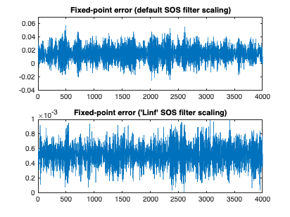
多くの場合、無限大ノルム SOS スケーリングで出力を生成することで誤差が少なくなります。
fig1 = figure;
subplot(3,1,1);
plot(out_1);
title('Floating-point filter output');
subplot(3,1,2);
plot(out_4);
title('Fixed-point (Linf-norm SOS) filter output');
subplot(3,1,3);
plot(out_1 - double(out_4));
axis([0 4000 0 1e-3]);
title('Error');

fig2 = figure;
subplot(2,1,1);
plot(out_1 - double(out_3));
axis([0 4000 -4e-2 7e-2]);
title('Fixed-point error (default SOS filter scaling)');
subplot(2,1,2);
plot(out_1 - double(out_4));
axis([0 4000 0 1e-3]);
title('Fixed-point error (''Linf'' SOS filter scaling)');
close(fig1); % clean up
close(fig2); % clean up
まとめ
ここでは、浮動小数点 IIR フィルターを固定小数点実装に変換する手順を説明しました。DSP System Toolbox™ の dsp.BiquadFilter オブジェクトには、シミュレーションの最小値と最大値のインストルメンテーション機能が備えられており、固定小数点コンバーター アプリで自動的かつ動的に内部フィルター信号をスケーリングするのに役立ちます。また、'fvtool' および spectrumAnalyzer は、さまざまな解析においてプロセスの各ステップで検証を行うためのツールとして使用できます。
You can also select a web site from the following list:
Americas
- América Latina (Español)
- Canada (English)
- United States (English)
Europe
- Belgium (English)
- Denmark (English)
- Deutschland (Deutsch)
- España (Español)
- Finland (English)
- France (Français)
- Ireland (English)
- Italia (Italiano)
- Luxembourg (English)
- Netherlands (English)
- Norway (English)
- Österreich (Deutsch)
- Portugal (English)
- Sweden (English)
- Switzerland
- United Kingdom (English)