このページの内容は最新ではありません。最新版の英語を参照するには、ここをクリックします。
CWT による時間-周波数解析
この例では、連続ウェーブレット変換 (CWT) を使用して信号を時間と周波数で一緒に解析する方法を示します。この例では、CWT が短時間フーリエ変換 (STFT) よりも優れている過渡特性の位置推定について説明します。また、この例では、逆 CWT を使用して時間-周波数局在型の信号 Approximation を合成する方法も示します。
CWT は多くの例で STFT と比較されます。spectrogram の例を実行するには、Signal Processing Toolbox™ がなければなりません。
変調信号の時間-周波数解析
二次チャープ信号を読み込みます。補助関数 helperCWTTimeFreqPlot を使用して、そのスペクトログラムのプロットを表示します。信号の周波数は t = 0 で約 500 Hz から始まり、t=2 で 100 Hz まで減少して、t=4 で再び 500 Hz まで増加します。サンプリング周波数は 1 kHz です。補助関数のコードは、この例のファイルと同じディレクトリにあります。
load quadchirp
fs = 1000;
[S,F,T] = spectrogram(quadchirp,100,98,128,fs);
helperCWTTimeFreqPlot(S,T,F, ...
    'surf','STFT of Quadratic Chirp','Seconds','Hz')

CWT を使用してこの信号の時間-周波数プロットを求めます。
[cfs,f] = cwt(quadchirp,fs,'WaveletParameters',[14,200]);
helperCWTTimeFreqPlot(cfs,tquad,f, ...
    'surf','CWT of Quadratic Chirp','Seconds','Hz')

Bump ウェーブレットを使用した CWT は STFT と非常に類似した時間-周波数解析を生成します。
周波数変調と振幅変調は自然信号で頻繁に発生します。CWT を使用して、オオクビワコウモリ (Eptesicus Fuscus) が発する反響定位パルスの時間-周波数解析を求めます。サンプリング間隔は 7 マイクロ秒です。オクターブあたりの音の数が 32 の Bump ウェーブレットを使用します。この例では、イリノイ大学 Beckman Center の Curtis Condon 氏、Ken White 氏、Al Feng 氏にコウモリのデータの提供および使用許可をいただきました。ご協力に謝意を申し上げます。
load batsignal
t = 0:DT:(numel(batsignal)*DT)-DT;
[cfs,f] = cwt(batsignal,'bump',1/DT,'VoicesPerOctave',32);
helperCWTTimeFreqPlot(cfs,t*1e6,f./1000, ...
    'surf','CWT of Bat Echolocation','Microseconds','kHz')

コウモリのデータの STFT を求めてプロットします。
[S,F,T] = spectrogram(batsignal,50,48,128,1/DT);
helperCWTTimeFreqPlot(S,T.*1e6,F./1e3, ...
    'surf','Bat Echolocation (STFT)','Microseconds','kHz')

シミュレーション信号と自然変調信号の両方について、CWT は STFT と類似した結果を提供します。
CWT を使用した振動の過渡特性の検出
時間-周波数解析には、短時間フーリエ変換よりも情報量の多い時間-周波数変換を CWT が提供できる特定の状況があります。この状況の 1 つは、信号が過渡特性によって破損した場合に発生します。これらの過渡特性の出現と消失には多くの場合、物理的な意味があります。したがって、信号における振動成分の特徴付けに加えて、これらの過渡特性の位置を特定できることが重要です。これをシミュレートするには、周波数 150 Hz および 200 Hz の 2 つの正弦波で構成される信号を作成します。サンプリング周波数は 1 kHz です。正弦波は互いに素の時間サポートをもちます。150 Hz の正弦波は 100 ~ 300 ミリ秒で発生します。200 Hz の正弦波は 700 ミリ秒~ 1 秒で発生します。さらに、222 ミリ秒と 800 ミリ秒に 2 つの過渡特性があります。信号はノイズによって破損します。
rng default
dt = 0.001;
t = 0:dt:1-dt;
addNoise = 0.025*randn(size(t));
x = cos(2*pi*150*t).*(t>=0.1 & t<0.3)+sin(2*pi*200*t).*(t>0.7);
x = x+addNoise;
x([222 800]) = x([222 800 ])+[-2 2];
%figure;
plot(t.*1000,x)
xlabel('Milliseconds')
ylabel('Amplitude')

この 2 つの過渡特性を拡大し、これらが 150 Hz と 200 Hz の振動で外乱を表していることを確認します。
subplot(2,1,1)
plot(t(184:264).*1000,x(184:264))
ylabel('Amplitude')
title('Transients')
axis tight
subplot(2,1,2)
plot(t(760:840).*1000,x(760:840))
ylabel('Amplitude')
axis tight
xlabel('Milliseconds')

解析 Morlet ウェーブレットを使用し、CWT を求めてプロットします。
figure
[cfs,f] = cwt(x,1/dt,'amor');
contour(t*1000,f,abs(cfs))
grid on
c = colorbar;
xlabel('Milliseconds')
ylabel('Frequency')
c.Label.String = 'Magnitude';

解析 Morlet ウェーブレットでは、Bump ウェーブレットよりも周波数の位置推定は劣化しますが、時間の位置推定は優れています。したがって、Morlet ウェーブレットの方が過渡特性の位置推定に適しています。振幅二乗の細かいスケール係数をプロットし、過渡特性の位置推定を示します。
figure
wt = cwt(x,1/dt,'amor');
plot(t.*1000,abs(wt(1,:)).^2)
xlabel('Milliseconds')
ylabel('Magnitude')
grid on
title('Analytic Morlet Wavelet -- Fine Scale Coefficients');

%hold offウェーブレットは、圧縮して精度の高い過渡特性の時間の局所化を有効にする一方、伸張して 150 Hz と 200 Hz における振動の周波数の局所化を許容します。
STFT はウィンドウの幅に対してのみ過渡特性の位置を特定することができます。STFT をデシベル (dB) 単位でプロットし、過渡特性を可視化できるようにしなければなりません。
[S,F,T] = spectrogram(x,50,48,128,1000);
surf(T.*1000,F,20*log10(abs(S)),'edgecolor','none')
view(0,90)
axis tight
shading interp
colorbar
xlabel('Time')
ylabel('Hz')
title('STFT')

過渡特性は、パワーの広帯域での増加としてのみ STFT に出現します。STFT から求められた短時間のパワー推定値を、最初の過渡特性が出現する前 (183 msec を中心とする) と後 (223 msec を中心とする) で比較します。
figure
plot(F,20*log10(abs(S(:,80))))
hold on
plot(F,20*log10(abs(S(:,100))),'r')
hold off
legend('T = 183 msec','T = 223 msec')
xlabel('Hz')
ylabel('dB')
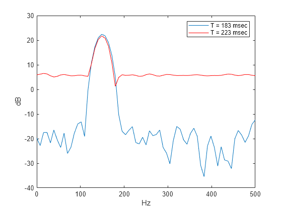
STFT は、CWT と同じレベルで過渡特性の位置を特定することはできません。
逆 CWT を使用した時間局在型の周波数成分の削除
指数的に重み付けされた正弦波で構成される信号を作成します。25 Hz 成分は、0.2 秒を中心としたものと 0.5 秒を中心としたものの 2 つあります。70 Hz 成分は、0.2 秒を中心としたものと 0.8 秒を中心としたものの 2 つあります。最初の 25 Hz 成分と 70 Hz 成分は同時に発生します。
t = 0:1/2000:1-1/2000;
dt = 1/2000;
x1 = sin(50*pi*t).*exp(-50*pi*(t-0.2).^2);
x2 = sin(50*pi*t).*exp(-100*pi*(t-0.5).^2);
x3 = 2*cos(140*pi*t).*exp(-50*pi*(t-0.2).^2);
x4 = 2*sin(140*pi*t).*exp(-80*pi*(t-0.8).^2);
x = x1+x2+x3+x4;
figure
plot(t,x)
title('Superimposed Signal')
CWT を求めて表示します。
cwt(x,2000)
title('Analytic CWT using Default Morse Wavelet');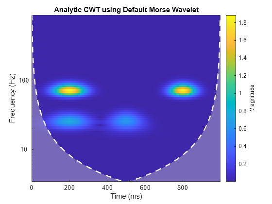
CWT 係数をゼロにして、約 0.07 ~ 0.3 秒の間に発生する 25 Hz 成分を削除します。逆 CWT (icwt) を使用し、信号の Approximation を再構成します。
[cfs,f] = cwt(x,2000);
T1 = .07;  T2 = .33;
F1 = 19;   F2 = 34;
cfs(f > F1 & f < F2, t> T1 & t < T2) = 0;
xrec = icwt(cfs);
再構成された信号の CWT を表示します。初期の 25 Hz 成分が削除されています。
cwt(xrec,2000)

元の信号と再構成したものをプロットします。
subplot(2,1,1)
plot(t,x)
title('Original Signal')
subplot(2,1,2)
plot(t,xrec)
title('Signal with first 25-Hz component removed')

最後に、0.2 秒を中心とした 25 Hz 成分を含めずに、再構成された信号を元の信号と比較します。
y = x2+x3+x4;
figure
plot(t,xrec)
hold on
plot(t,y,'r--')
hold off
legend('Inverse CWT approximation','Original signal without 25-Hz')

解析 CWT による正確な周波数の決定
解析ウェーブレットを使用して正弦波のウェーブレット変換を求めると、解析 CWT 係数は実際に周波数を符号化します。
これを説明するために、人間の耳から得られる耳音響放射について考えます。耳音響放射 (OAE) は蝸牛 (内耳) から発せられ、これがあることは正常な聴力を示します。OAE データを読み込んでプロットします。データは 20 kHz でサンプリングされます。
load dpoae
plot(t.*1000,dpoaets)
xlabel('Milliseconds')
ylabel('Amplitude')

この放射は 25 ミリ秒から開始して 175 ミリ秒で終了するスティミュラスによって誘発されました。実験パラメーターに基づき、放射の周波数は 1230 Hz になります。CWT を求めてプロットします。
cwt(dpoaets,'bump',20000)
xlabel('Milliseconds')

OAE の時間発展は、周波数が 1230 Hz に最も近い CWT 係数を求め、その振幅を時間の関数として調べることで検証できます。誘発スティミュラスの開始と終了を指定する時間マーカーと共に振幅をプロットします。
[dpoaeCWT,f] = cwt(dpoaets,'bump',20000);
[~,idx1230] = min(abs(f-1230));
cfsOAE = dpoaeCWT(idx1230,:);
plot(t.*1000,abs(cfsOAE))
hold on
AX = gca;
plot([25 25],[AX.YLim(1) AX.YLim(2)],'r')
plot([175 175],[AX.YLim(1) AX.YLim(2)],'r')
hold off
xlabel('Milliseconds')
ylabel('Magnitude')
title('CWT Coefficient Magnitudes')

誘発スティミュラスのオンセットと OAE との間にいくらかの遅延があります。誘発スティミュラスが終了すると、OAE はすぐに振幅が減衰し始めます。
放射を分離するもう 1 つの方法は、逆 CWT を使用して時間領域で周波数局在型の Approximation を再構成することです。
周波数範囲 [1150 1350] Hz で逆 CWT を行い、周波数局在型の放射の Approximation を再構成します。誘発スティミュラスの開始と終了を示す再構成とマーカーと共に元のデータをプロットします。
xrec = icwt(dpoaeCWT,'bump',f,[1150 1350]);
%figure
plot(t.*1000,dpoaets)
hold on
plot(t.*1000,xrec,'r')
AX = gca;
ylim = AX.YLim;
plot([25 25],ylim,'k')
plot([175 175],ylim,'k')
hold off
xlabel('Milliseconds')
ylabel('Amplitude')
title('Frequency-Localized Reconstruction of Emission')

時間領域データでは、誘発スティミュラスの適用時と終了時に放射が増減するようすをはっきりと確認できます。
ここで重要な点は、再構成には周波数の範囲が選択された場合でも、解析ウェーブレット変換は実際には放射の正確な周波数を符号化することです。これを示すために、解析 CWT から再構成された放射の Approximation のフーリエ変換を使用します。
xdft = fft(xrec);
freq = 0:2e4/numel(xrec):1e4;
xdft = xdft(1:numel(xrec)/2+1);
figure
plot(freq,abs(xdft))
xlabel('Hz')
ylabel('Magnitude')
title('Fourier Transform of CWT-Based Signal Approximation')

[~,maxidx] = max(abs(xdft));
fprintf('The frequency is %4.2f Hz.\n',freq(maxidx));
The frequency is 1230.00 Hz.
まとめ
この例では、CWT を使用して cwt で解析ウェーブレットを使用した 1 次元信号の時間-周波数解析を求める方法について説明しました。CWT が STFT と類似した結果を提供する信号の例と、CWT が STFT より解釈しやすい結果を提供できる例を確認しました。最後に、icwt を使用して時間-スケール (周波数) 局在型の Approximation を信号に再構成する方法を確認しました。
参照
[1] Mallat, S. G. A Wavelet Tour of Signal Processing: The Sparse Way. 3rd ed. Amsterdam ; Boston: Elsevier/Academic Press, 2009.
参考
アプリ
関数
オブジェクト
関連するトピック
You can also select a web site from the following list:
Americas
- América Latina (Español)
- Canada (English)
- United States (English)
Europe
- Belgium (English)
- Denmark (English)
- Deutschland (Deutsch)
- España (Español)
- Finland (English)
- France (Français)
- Ireland (English)
- Italia (Italiano)
- Luxembourg (English)
- Netherlands (English)
- Norway (English)
- Österreich (Deutsch)
- Portugal (English)
- Sweden (English)
- Switzerland
- United Kingdom (English)