Nonclassical and Nonmetric Multidimensional Scaling
Perform nonclassical multidimensional scaling using mdscale.
Nonclassical Multidimensional Scaling
The function mdscale performs nonclassical multidimensional scaling. As with cmdscale, you use mdscale either to visualize dissimilarity data for which no “locations” exist, or to visualize high-dimensional data by reducing its dimensionality. Both functions take a matrix of dissimilarities as an input and produce a configuration of points. However, mdscale offers a choice of different criteria to construct the configuration, and allows missing data and weights.
For example, the cereal data include measurements on 10 variables describing breakfast cereals. You can use mdscale to visualize these data in two dimensions. First, load the data. For clarity, this example code selects a subset of 22 of the observations.
load cereal.mat
X = [Calories Protein Fat Sodium Fiber ...
    Carbo Sugars Shelf Potass Vitamins];
% Take a subset from a single manufacturer
mfg1 = strcmp('G',cellstr(Mfg));
X = X(mfg1,:);
size(X)
ans =
    22 10
Then use pdist to transform the 10-dimensional data into dissimilarities. The output from pdist is a symmetric dissimilarity matrix, stored as a vector containing only the (23*22/2) elements in its upper triangle.
dissimilarities = pdist(zscore(X),'cityblock');
size(dissimilarities)
ans =
     1   231
This example code first standardizes the cereal data, and then uses city block distance as a dissimilarity. The choice of transformation to dissimilarities is application-dependent, and the choice here is only for simplicity. In some applications, the original data are already in the form of dissimilarities.
Next, use mdscale to perform metric MDS. Unlike cmdscale, you must specify the desired number of dimensions, and the method to use to construct the output configuration. For this example, use two dimensions. The metric STRESS criterion is a common method for computing the output; for other choices, see the mdscale reference page in the online documentation. The second output from mdscale is the value of that criterion evaluated for the output configuration. It measures the how well the inter-point distances of the output configuration approximate the original input dissimilarities:
[Y,stress] =...
mdscale(dissimilarities,2,'criterion','metricstress');
stress
stress =
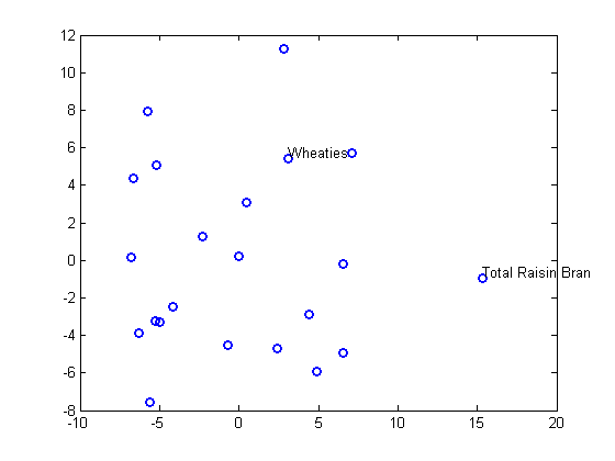
0.1856A scatterplot of the output from mdscale represents the original 10-dimensional data in two dimensions, and you can use the gname function to label selected points:
plot(Y(:,1),Y(:,2),'o','LineWidth',2);
gname(Name(mfg1))
Nonmetric Multidimensional Scaling
Metric multidimensional scaling creates a configuration of points whose inter-point distances approximate the given dissimilarities. This is sometimes too strict a requirement, and non-metric scaling is designed to relax it a bit. Instead of trying to approximate the dissimilarities themselves, non-metric scaling approximates a nonlinear, but monotonic, transformation of them. Because of the monotonicity, larger or smaller distances on a plot of the output will correspond to larger or smaller dissimilarities, respectively. However, the nonlinearity implies that mdscale only attempts to preserve the ordering of dissimilarities. Thus, there may be contractions or expansions of distances at different scales.
You use mdscale to perform nonmetric MDS in much the same way as for metric scaling. The nonmetric STRESS criterion is a common method for computing the output; for more choices, see the mdscale reference page in the online documentation. As with metric scaling, the second output from mdscale is the value of that criterion evaluated for the output configuration. For nonmetric scaling, however, it measures the how well the inter-point distances of the output configuration approximate the disparities. The disparities are returned in the third output. They are the transformed values of the original dissimilarities:
[Y,stress,disparities] = ...
mdscale(dissimilarities,2,'criterion','stress');
stress
stress =
    0.1562
To check the fit of the output configuration to the dissimilarities, and to understand the disparities, it helps to make a Shepard plot:
distances = pdist(Y);
[dum,ord] = sortrows([disparities(:) dissimilarities(:)]);
plot(dissimilarities,distances,'bo', ...
     dissimilarities(ord),disparities(ord),'r.-', ...
     [0 25],[0 25],'k-')
xlabel('Dissimilarities')
ylabel('Distances/Disparities')
legend({'Distances' 'Disparities' '1:1 Line'},...
       'Location','NorthWest');
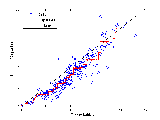
This plot shows that mdscale has found a configuration of points in two dimensions whose inter-point distances approximates the disparities, which in turn are a nonlinear transformation of the original dissimilarities. The concave shape of the disparities as a function of the dissimilarities indicates that fit tends to contract small distances relative to the corresponding dissimilarities. This may be perfectly acceptable in practice.
mdscale uses an iterative algorithm to find the output configuration, and the results can often depend on the starting point. By default, mdscale uses cmdscale to construct an initial configuration, and this choice often leads to a globally best solution. However, it is possible for mdscale to stop at a configuration that is a local minimum of the criterion. Such cases can be diagnosed and often overcome by running mdscale multiple times with different starting points. You can do this using the 'start' and 'replicates' name-value pair arguments. The following code runs five replicates of MDS, each starting at a different randomly-chosen initial configuration. The criterion value is printed out for each replication; mdscale returns the configuration with the best fit.
opts = statset('Display','final');
[Y,stress] =...
mdscale(dissimilarities,2,'criterion','stress',...
'start','random','replicates',5,'Options',opts);
35 iterations, Final stress criterion = 0.156209
31 iterations, Final stress criterion = 0.156209
48 iterations, Final stress criterion = 0.171209
33 iterations, Final stress criterion = 0.175341
32 iterations, Final stress criterion = 0.185881
Notice that mdscale finds several different local solutions, some of which do not have as low a stress value as the solution found with the cmdscale starting point.
See Also
You can also select a web site from the following list:
Americas
- América Latina (Español)
- Canada (English)
- United States (English)
Europe
- Belgium (English)
- Denmark (English)
- Deutschland (Deutsch)
- España (Español)
- Finland (English)
- France (Français)
- Ireland (English)
- Italia (Italiano)
- Luxembourg (English)
- Netherlands (English)
- Norway (English)
- Österreich (Deutsch)
- Portugal (English)
- Sweden (English)
- Switzerland
- United Kingdom (English)