Examining Residuals for Model Verification
You can examine the stats structure, which is returned by both nlmefit and nlmefitsa, to determine the quality of your model. The stats structure contains fields with conditional weighted residuals (cwres field) and individual weighted residuals (iwres field). Since the model assumes that residuals are normally distributed, you can examine the residuals to see how well this assumption holds.
This example generates synthetic data using normal distributions. It shows how the fit statistics look:
Good when testing against the same type of model as generates the data
Poor when tested against incorrect data models
1. Initialize a 2-D model with 100 individuals.
nGroups = 100; % 100 Individuals
nlmefun = @(PHI,t)(PHI(:,1)*5 + PHI(:,2)^2.*t); % Regression fcn
REParamsSelect = [1  2]; % Both Parameters have random effect
errorParam = .03;
beta0 = [ 1.5  5]; % Parameter means
psi = [ 0.35  0; ...  % Covariance Matrix
    0   0.51 ];
time =[0.25;0.5;0.75;1;1.25;2;3;4;5;6];
nParameters = 2;
rng(0,'twister') % for reproducibility
2. Generate the data for fitting with a proportional error model.
b_i = mvnrnd(zeros(1, numel(REParamsSelect)), psi, nGroups);
individualParameters = zeros(nGroups,nParameters);
individualParameters(:, REParamsSelect) = ...
    beta0(REParamsSelect) + b_i;

groups = repmat(1:nGroups,numel(time),1);
groups = vertcat(groups(:));

y = zeros(numel(time)*nGroups,1);
x = zeros(numel(time)*nGroups,1);
for i = 1:nGroups
    idx = groups == i;
    f = nlmefun(individualParameters(i,:), time);
    % Make a proportional error model for y:
    y(idx) = f + errorParam*f.*randn(numel(f),1);
    x(idx) = time;
end

P = [ 1 0 ; 0 1 ];
3. Fit the data using the same regression function and error model as the model generator.
[~,~,stats] = nlmefit(x,y,groups, ...
    [],nlmefun,[1 1],'REParamsSelect',REParamsSelect,...
    'ErrorModel','Proportional','CovPattern',P);
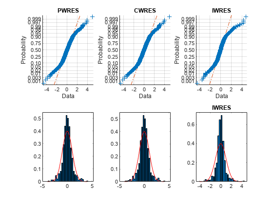
4. Plot the residuals using the helper function helper_plotResiduals function. The code for the helper_plotResiduals function appears at the end of this example.
helper_plotResiduals(stats)

The upper probability plots look straight, meaning the residuals are normally distributed. The bottom histogram plots match the superimposed normal density plot. So you can conclude that the error model matches the data.
5. For comparison, fit the data using a constant error model, instead of the proportional model that created the data.
[~,~,stats] = nlmefit(x,y,groups, ...
    [],nlmefun,[0 0],'REParamsSelect',REParamsSelect,...
    'ErrorModel','Constant','CovPattern',P);
helper_plotResiduals(stats)
The upper probability plots are not straight, indicating the residuals are not normally distributed. The bottom histogram plots are fairly close to the superimposed normal density plots.
6. For another comparison, fit the data to a different structural model than the one that created the data.
nlmefun2 = @(PHI,t)(PHI(:,1)*5 + PHI(:,2).*t.^4);
[~,~,stats] = nlmefit(x,y,groups, ...
    [],nlmefun2,[0 0],'REParamsSelect',REParamsSelect,...
    'ErrorModel','constant', 'CovPattern',P);
helper_plotResiduals(stats)

The upper probability plots are not straight. Also, the histogram plots are quite skewed compared to the superimposed normal density plots. These residuals are not normally distributed, and do not match the model.
Helper Function
function helper_plotResiduals(stats)
pwres = stats.pwres;
iwres = stats.iwres;
cwres = stats.cwres;
figure
subplot(2,3,1);
normplot(pwres); title('PWRES')
subplot(2,3,4);
createhistplot(pwres);

subplot(2,3,2);
normplot(cwres); title('CWRES')
subplot(2,3,5);
createhistplot(cwres);

subplot(2,3,3);
normplot(iwres); title('IWRES')
subplot(2,3,6);
createhistplot(iwres); title('IWRES')

    function createhistplot(pwres)
        h = histogram(pwres);

        % x is the probability/height for each bin
        x = h.Values/sum(h.Values*h.BinWidth);

        % n is the center of each bin
        n = h.BinEdges + (0.5*h.BinWidth);
        n(end) = [];

        bar(n,x);
        ylim([0 max(x)*1.05]);
        hold on;
        x2 = -4:0.1:4;
        f2 = normpdf(x2,0,1);
        plot(x2,f2,'r');
    end

end
See Also
Related Topics
You can also select a web site from the following list:
Americas
- América Latina (Español)
- Canada (English)
- United States (English)
Europe
- Belgium (English)
- Denmark (English)
- Deutschland (Deutsch)
- España (Español)
- Finland (English)
- France (Français)
- Ireland (English)
- Italia (Italiano)
- Luxembourg (English)
- Netherlands (English)
- Norway (English)
- Österreich (Deutsch)
- Portugal (English)
- Sweden (English)
- Switzerland
- United Kingdom (English)