不等間隔サンプル信号のリサンプリング

不等間隔サンプル信号の目的のレートへのリサンプリング

関数 resample では、不等間隔サンプル信号を新しい等間隔のレートに変換できます。

約 48 kHz で不規則にサンプリングされた 500 Hz の正弦波を作成します。乱数値を均一なベクトルに加えることで不規則性をシミュレートします。

rng default
nominalFs = 48000;
f = 500;
Tx = 0:1/nominalFs:0.01;
irregTx = sort(Tx + 1e-4*rand(size(Tx)));
x = sin(2*pi*f*irregTx);
plot(irregTx,x,'.')

不等間隔サンプル信号をリサンプリングするには、時間ベクトル入力を指定して resample を呼び出します。

次の例では、元の信号が 44.1 kHz の等間隔のレートに変換されます。

desiredFs = 44100;
[y, Ty] = resample(x,irregTx,desiredFs);
plot(irregTx,x,'.-',Ty,y,'o-')
legend('Original','Resampled')
ylim([-1.2 1.2])

リサンプリングした信号の形状とサイズが元の信号と同じであることが確認できます。

内挿法の選択

resample の変換アルゴリズムは、入力サンプルが等間隔に近ければ近いほど適切に機能します。そのため、サンプリングされたデータから入力サンプルの一部が欠けた場合にどうなるかを観察すると有益です。

次の例では、入力正弦波の 2 番目の波高をノッチ フィルターで低減し、リサンプリングを適用します。

irregTx(105:130) = [];
x = sin(2*pi*f*irregTx);
[y, Ty] = resample(x,irregTx,desiredFs);

plot(irregTx,x,'. ')
hold on
plot(Ty,y,'.-')
hold off
legend('Original','Resampled')
ylim([-1.2 1.2])

セグメントの欠損部は線形内挿によってつなげられます。関数 resample で不等間隔サンプル データをリサンプリングする場合には、既定の方法として線形内挿が使用されます。

データの欠損がある場合や入力内の隙間が大きい場合などには、別の内挿法を選択して欠損データを部分的に復元できます。

低ノイズ、低帯域幅の信号では、元の信号の再構成にスプラインを使用すると非常に効果的です。リサンプリングの際に 3 次スプラインを使用するには、'spline' 内挿法を指定します。

[y, Ty] = resample(x,irregTx,desiredFs,'spline');

plot(irregTx,x,'. ')
hold on
plot(Ty,y,'.-')
hold off
legend('Original','Resampled using ''spline''')
ylim([-1.2 1.2])

内挿グリッドの制御

既定の設定では、resample は、目的のサンプル レートと信号の平均サンプル レートの比率の密な有理近似である中間グリッドを構成します。

入力サンプルの一部に高周波数成分が含まれている場合、整数の係数 p および q を選んでこの有理数比率を選択することで、中間グリッドの間隔を制御することができます。

約 3 Hz のレートで振動する不足減衰 2 次フィルターのステップ応答を調べます。

w = 2*pi*3;
d = .1002;
z = sin(d);
a = cos(d); 

t = [0:0.05:2 3:8];

x = 1 - exp(-z*w*t).*cos(w*a*t-d)/a;
plot(t,x,'.-')

ステップ応答は、振動している高レートおよび振動していない低レートでサンプリングされます。

ここで、既定の設定をそのまま使用して、信号を 100 Hz でリサンプリングします。

Fs = 100;
[y, Ty] = resample(x,t,Fs);
plot(t,x,'. ')
hold on
plot(Ty,y)
hold off
legend('Original','Resampled (default settings)')

波形の開始点で振動の包絡線が減衰され、元の信号よりゆっくり振動するようになります。

既定の設定では、resample は入力信号の平均サンプル レートに対応する一定間隔のグリッドに内挿します。

avgFs = (numel(t)-1) /(t(end)-t(1))

avgFs = 5.7500

グリッドのサンプル レートは、測定しようとする最大周波数の 2 倍超の高さである必要があります。このグリッドのサンプル レートは 1 秒あたり 5.75 サンプルで、ナイキストのサンプル レートである、リンギング周波数の 6 Hz より低くなっています。

グリッドのサンプル レートを上げるには、整数パラメーター p および q を指定します。resample は、グリッドのサンプル レートを Q*Fs/P に調節してから内部サンプル レート変換器 (P によるアップサンプリングおよび Q によるダウンサンプリング) を適用し、目的のサンプル レート Fs を復元します。rat を使用し、p および q を選択します。

振動のリンギングが 3 Hz であるため、グリッドには 7 Hz のサンプル レートを指定します。これは、ナイキスト レートより少し高くなっています。1 Hz のヘッドルームは、指数エンベロープが減衰するために追加の周波数成分に相当します。

Fgrid = 7;
[p,q] = rat(Fs/Fgrid)

p = 100

q = 7

[y, Ty] = resample(x,t,Fs,p,q);
plot(t,x,'.')
hold on
plot(Ty,y)
hold off
legend('Original','Resampled (custom P and Q)')

アンチエイリアシング フィルターの指定

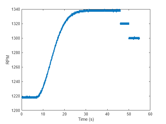
次の例では、飛行機のエンジンのスロットル設定を測定するデジタイザーの出力を表示します。スロットル設定は、約 100 Hz のノミナル レートで不等間隔にサンプリングされています。等間隔な 10 Hz のレートでこの信号をリサンプリングします。

以下は元の信号のサンプルです。

load engineRPM
plot(t,x,'.')
xlabel('Time (s)')
ylabel('RPM')

信号は量子化されています。ここで、20 秒から 23 秒の時間区間の上昇領域を拡大します。

plot(t,x,'.')
xlim([20 23])

信号はこの領域内でゆっくり変化しています。そのため、リサンプラーのアンチエイリアシング フィルターを使用して量子化ノイズの一部を除去できます。

desiredFs = 10;
[y,ty] = resample(x,t,desiredFs);

plot(t,x,'.')
hold on
plot(ty,y,'.-')
hold off
xlabel('Time')
ylabel('RPM')
legend('Original','Resampled')
xlim([20 23])

これは、かなりの効果があります。しかし、カットオフ周波数の低い resample フィルターを使用することで、リサンプリングされた信号をさらに平滑化できます。

最初に、グリッドの間隔がノミナル サンプル レートである約 100 Hz になるように設定します。

nominalFs = 100;

次に、目的のレートを取得するのに適切な p および q を決定します。ノミナル レートが 100 Hz で目的のレートが 10 Hz であるため、10 で間引く必要があります。これは p を 1、q を 10 に設定することに相当します。

p = 1;
q = 10;

独自のフィルターを resample に指定できます。適切に時間調節するために、フィルターは奇数長である必要があります。フィルターの長さは p または q (大きい方) の数倍でなければなりません。目的とするカットオフの 1 / q となるようにカットオフ周波数を設定し、次に結果として得られる係数を p で乗算します。

% ensure an odd length filter
n = 10*q+1;

% use .25 of Nyquist range of desired sample rate
cutoffRatio = .25;

% construct lowpass filter 
lpFilt = p * fir1(n, cutoffRatio * 1/q);

% resample and plot the response
[y,ty] = resample(x,t,desiredFs,p,q,lpFilt);

plot(t,x,'.')
hold on
plot(ty,y)
hold off
xlabel('time')
ylabel('RPM')
legend('Original','Resampled (custom filter)','Location','best')
xlim([20 23])

端点の影響の除去

ズーム アウトして元の信号を表示します。端点にかなりのオフセットがあることに注意してください。

plot(t,x,'.',ty,y)
xlabel('time')
ylabel('RPM')
legend('original','resampled (custom filter)','Location','best')

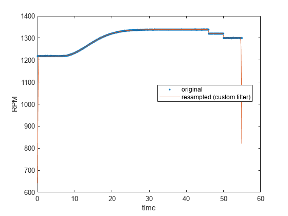
これらのアーティファクトは、resample が、信号はその境界線外ではゼロであると仮定することから発生します。これらの不連続部分の影響を低減するには、信号の端点間の線を除去してリサンプリングを実行した後、元の関数に線を追加し直します。最初と最後のサンプル間の線の勾配とオフセットを計算し、polyval を使用して除去する線を作成することで、これを実行できます。

% compute slope and offset (y = a1 x + a2)
a(1) = (x(end)-x(1)) / (t(end)-t(1));
a(2) = x(1);

% detrend the signal
xdetrend = x - polyval(a,t);
plot(t,xdetrend)

トレンド除去した信号の両方の端点がゼロに近くなりました。これで発生した過渡特性が抑制されます。resample を呼び出してから、トレンドを追加し直します。

[ydetrend,ty] = resample(xdetrend,t,desiredFs,p,q,lpFilt);

y = ydetrend + polyval(a,ty);

plot(t,x,'.',ty,y)
xlabel('Time')
ylabel('RPM')
legend('Original','Resampled (detrended, custom filter)','Location','best')

まとめ

この例では、resample を使用し、等間隔および不等間隔のサンプル信号を固定レートに変換する方法を説明しています。

参考情報

カスタム スプラインによる不等間隔サンプルの再構成の詳細については、Curve Fitting Toolbox™ のドキュメンテーションを参照してください。