Wind-Powered Vehicle with Propeller

Open Live Script

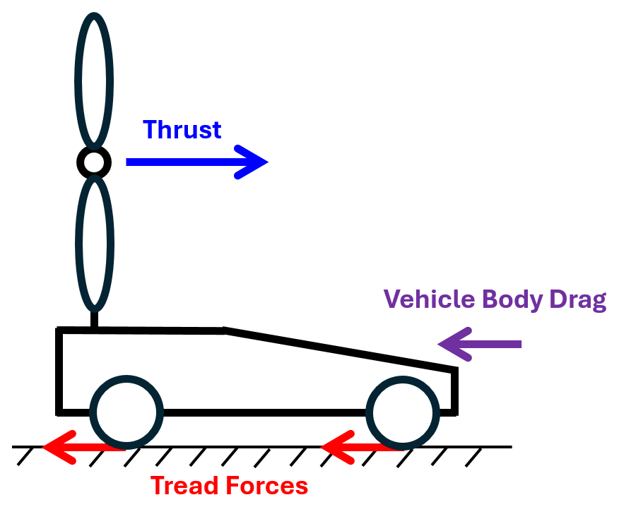
This example shows a wind-powered four-wheel vehicle with a propeller that travels faster than the wind speed. The wind blows from the rear to the front of the vehicle, and the propeller thrust is the driving force. The forces acting on the vehicle are the propeller thrust, the vehicle body drag, and the tread forces. When the vehicle speed exceeds the wind speed, the body experiences a drag force. The vehicle travels faster than the wind speed because the thrust force overcomes the drag and tread forces. The figure shows the directions of the forces exerted on the vehicle.

Model

The example model represents a vehicle that consists of a propeller, a vehicle body, a driveshaft, a gear box, and four wheels. The propeller connects to the driveshaft through the gear box. The four wheels and driveshaft have rotational inertias, and the vehicle body has an associated mass. The gear box imposes a kinematic constraint between the angular velocities of the propeller and the driveshaft with a fixed gear ratio. This constraint makes the propeller rotate and displace air from front to rear as the wheels rotate in the direction advancing the vehicle. The propeller displacing air from front to rear is subject to an aerodynamic torque, and the kinematic constraint makes this torque hinder the advance of vehicle. The initial model uses an Aerodynamic Propeller block parameterized by Tabulated data for advance angle. Open the model.

open_system("WindPoweredVehicleWithPropeller");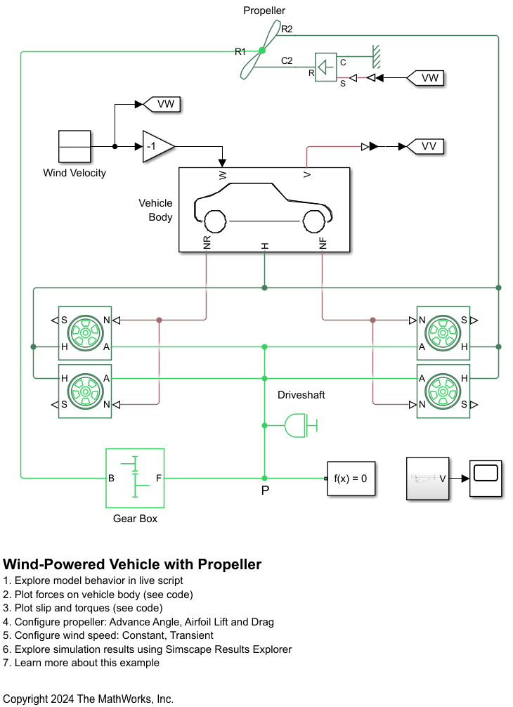

Constant Wind Velocity

The initial model specifies the wind speed to 10 m/s. Double-click the Wind Velocity block.

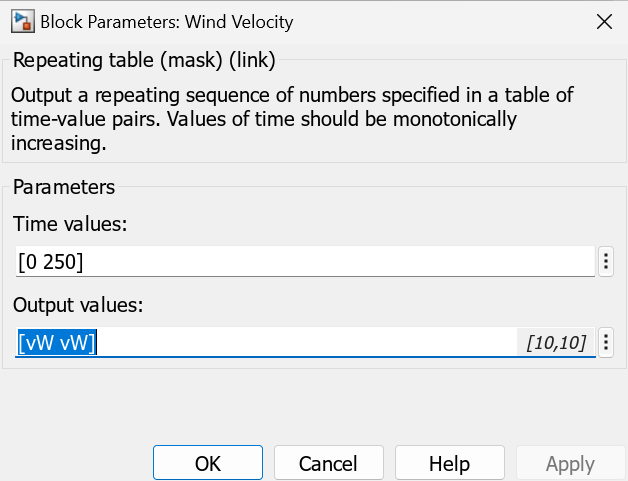
Run the model. The vehicle velocity exceeds the wind velocity at 63 seconds.

sim("WindPoweredVehicleWithPropeller");                
open_system("WindPoweredVehicleWithPropeller/Scope");

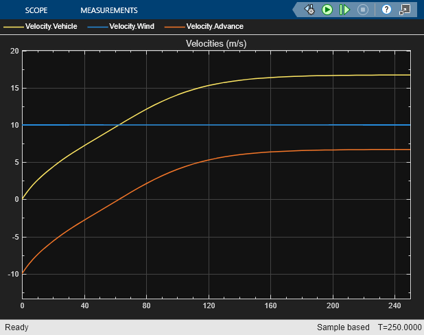
The advance velocity equals the vehicle velocity minus the wind velocity.

Forces and Torques

Plot the forces acting on the vehicle.

WindPoweredVehicleWithPropellerPlot1Forces

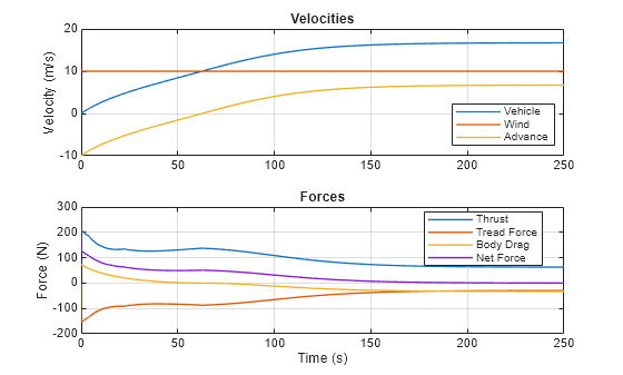
Figure WindPoweredVehicleWithPropeller contains 2 axes objects. Axes object 1 with title Velocities, ylabel Velocity (m/s) contains 3 objects of type line. These objects represent Vehicle, Wind, Advance. Axes object 2 with title Forces, xlabel Time (s), ylabel Force (N) contains 4 objects of type line. These objects represent Thrust, Tread Force, Body Drag, Net Force.

The Tread Force plot shows the sum of all tread forces to the wheels. Positive forces correspond to forward vehicle motion. The positive net force approaches to zero as the vehicle velocity approaches a steady-state.

Plot the wheel slip and the torque flow balance at the location P shown on the canvas. All wheels experience the same slip because they have the same angular velocity and radius. The wheels are modeled using Tire (Magic Formula) blocks.

WindPoweredVehicleWithPropellerPlot2Slip

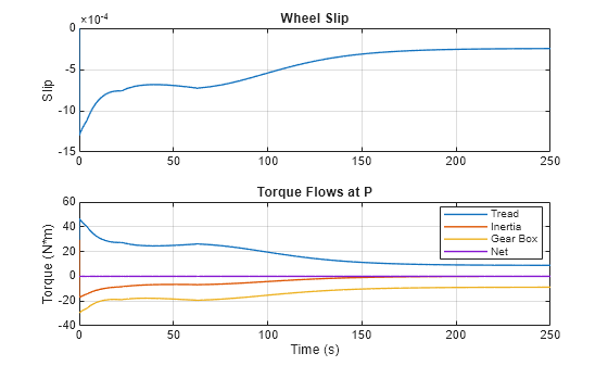
Figure WindPoweredVehicleWithPropeller contains 2 axes objects. Axes object 1 with title Wheel Slip, ylabel Slip contains an object of type line. Axes object 2 with title Torque Flows at P, xlabel Time (s), ylabel Torque (N*m) contains 4 objects of type line. These objects represent Tread, Inertia, Gear Box, Net.

The negative slip means that the vehicle velocity is greater than the wheel circumferential velocity, and the tread forces act to slow down the vehicle. These forces result in the tread torque that balances the torque provided to the gear box for the propeller as well as torques to accelerate wheels and the driveshaft. The net torque flow is always zero, and the gear box torque compensates the tread torque at the steady-state.

Advance Angle

When you set Parameterization to Tabulated data for advance angle, the Aerodynamic Propeller block uses uses quadrants to determine the thrust and torque coefficients from the advance angle. Plot the thrust coefficient $C_{T}$ and torque coefficient $C_{Q}$ vectors with respect to the advance angle vector. The magnitude of the thrust coefficient is typically much larger than that of the torque coefficient.

% Plot thrust and torque coefficient vectors
param_beta = str2num(get_param("WindPoweredVehicleWithPropeller/Propeller","beta_TLU"))';   % Advance angle vector (deg)
param_Ct = str2num(get_param("WindPoweredVehicleWithPropeller/Propeller","Ct_TLU_1D"))';    % Thrust coefficient vector
param_Cq = str2num(get_param("WindPoweredVehicleWithPropeller/Propeller","Cq_TLU_1D"))';    % Torque coefficient vector

figure, subplot(2,1,1);
plot(param_beta, [param_Ct, -10*param_Cq], "LineWidth", 1);
title("Thrust and Torque Coefficients")
xlabel("Advance Angle (deg)"); xlim([0 360]);
ylabel("Coefficient");
legend({"C_T","-10C_Q"}, "Location", "best");
grid on

Plot the advance angle.

simlog_t = simlog_WindPoweredVehicleWithPropeller.Propeller.beta.series.time;               % Time (s)
simlog_beta = simlog_WindPoweredVehicleWithPropeller.Propeller.beta.series.values("deg");   % Advance angle (deg)

subplot(2,1,2);
plot(simlog_t, simlog_beta, "LineWidth", 1);
title("Advance Angle");
xlabel("Time (s)"); xlim([0 simlog_t(end)]);
ylabel("Angle (deg)");
grid on

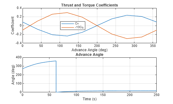
Figure contains 2 axes objects. Axes object 1 with title Thrust and Torque Coefficients, xlabel Advance Angle (deg), ylabel Coefficient contains 2 objects of type line. These objects represent C_T, -10C_Q. Axes object 2 with title Advance Angle, xlabel Time (s), ylabel Angle (deg) contains an object of type line.

The advance angle remains in the fourth quadrant (270 $°$ - 360 $°$ ) in the initial period when the vehicle has negative advance velocity and shifts to the first quadrant (0 $°$ - 90 $°$ ) when the vehicle velocity exceeds the wind velocity. The advance angle is 17 $°$ at the steady-state. Both coefficients are positive throughout the simulation.

Steady State Analysis

When the vehicle velocity reaches steady-state,

$\sum T r e a d F o r c e s + T h r u s t + B o d y D r a g = 0$

In the Gear Box block, the aerodynamic torque from the propeller balances the torques generated by tread forces.

$A e r o d y n a m i c T o r q u e \times G e a r R a t i o + W h e e l R a d i u s \times \sum T r e a d F o r c e s = 0$

Substitute the first equation into the second to obtain a steady-state relation.

$A e r o d y n a m i c T o r q u e = \frac{W h e e l R a d i u s}{G e a r R a t i o} \times (T h r u s t + B o d y D r a g)$

Plot the aerodynamic torque versus the thrust plus body drag, which represents possible driving conditions. Compare this plot to the stead state relation.

n = 0:0.1:3;                           % Propeller angular velocity (Hz)
vW = 10;                               % Wind speed (m/s)
vV = radiusWheel * (2*pi*n)/gearRatio; % Vehicle velocity (m/s) 
vA = vV - vW;                          % Advance velocity (m/s) 
vR_squared = vA.^2 + (0.7 * propDiameter * pi * n).^2;           % Relative advance velocity squared (m^2/s^2)
beta = wrapTo360(atan2(vA, 0.7*pi*n*propDiameter)/2/pi*360);     % Advance angle (deg)
torque = interp1(param_beta, param_Cq, beta, "linear", "extrap") ...
    * 1/8 * airDensity .* vR_squared * pi * propDiameter^3;                   % Torque (N*m)
thrust = interp1(param_beta, param_Ct, beta, "linear", "extrap") ...
    * 1/8 * airDensity .* vR_squared * pi * propDiameter^2;                   % Thrust (N)
drag = -1/2 * airDensity * dragCoeff * area * (vV - vW).^2 .* sign(vV - vW);  % Vehicle body drag (N)
figure, plot(thrust + drag, torque, "LineWidth", 1);
hold on;
plot(-50:1:50,radiusWheel/gearRatio*(-50:1:50), "LineWidth", 1);
xlabel("Thrust + Body Drag (N)"); xlim([-50 50]);
ylabel("Aerodynamic Torque (N*m)");
legend("Torque vs. (Thrust + Body Drag)", "Steady State Relation", "Location", "best");
title("Steady State Analysis");
grid on

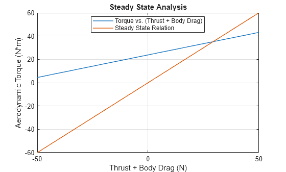
Figure contains an axes object. The axes object with title Steady State Analysis, xlabel Thrust + Body Drag (N), ylabel Aerodynamic Torque (N*m) contains 2 objects of type line. These objects represent Torque vs. (Thrust + Body Drag), Steady State Relation.

The intersecting point of the two curves is the steady-state solution. The coordinate of the interesection is

$(T h r u s t + B o d y D r a g, A e r o d y n a m i c T o r q u e) = (29, 35)$

Verify the coordinate with the simulation result.

torque = simlog_WindPoweredVehicleWithPropeller.Propeller.Q.series.values("N*m");
steadyStateTorque = torque(end);
disp("Aerodynamic torque at steady-state is " + steadyStateTorque + " N*m");

Aerodynamic torque at steady-state is 35.3149 N*m

The slope, $W h e e l R a d i u s / G e a r R a t i o$ , of the steady-state curve determines the location of the intersection. Increasing the slope of the curve causes the two curves to intersect at a lower aerodynamic torque. Increase the slope by changing the wheel radius from 0.3 m to 0.4 m and verify that the steady-state torque decreases.

radiusWheel = 0.4;
sim("WindPoweredVehicleWithPropeller");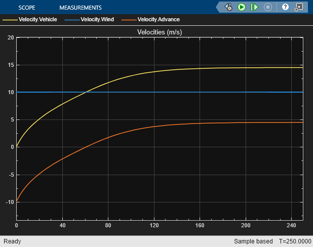

torque = simlog_WindPoweredVehicleWithPropeller.Propeller.Q.series.values("N*m");
steadyStateTorque = torque(end);
radiusWheel = 0.3;                      
disp("Aerodynamic torque at steady-state with the increased wheel radius is " + steadyStateTorque + " N*m");

Aerodynamic torque at steady-state with the increased wheel radius is 12.8656 N*m

Airfoil Lift and Drag Coefficients Parameterization

You can use a first-principle representation with the Aerodynamic Propeller block. Configure the propeller to use the Tabulated data for airfoil lift and drag coefficients parameterization. This parameterization specifies lift and drag coefficients over the radial distance of the blade and uses Blade Element Theory to obtain the thrust and torque exerted on the propeller.

set_param("WindPoweredVehicleWithPropeller/Propeller","parameterization","sdl.enum.AerodynamicPropellerParameterization.Airfoil") 
sim("WindPoweredVehicleWithPropeller")

Four-Quadrant Model from Lift and Drag Parameterization

Open the test rig model that contains an Aerodynamic Propeller block that is parameterized identically to the wind-powered vehicle Aerodynamic Propeller block.

open_system("WindPoweredVehicleWithPropellerTestRig");
sim("WindPoweredVehicleWithPropellerTestRig");

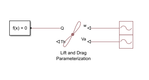
Derive an equivalent four-quadrant model using the test rig, which sweeps the advance angle from 0 $°$ to 360 $°$ .

simlog_nTest = simlog_WindPoweredVehicleWithPropellerTestRig.Lift_and_Drag_Parameterization.w_in.series.values("Hz");     % Angular velocity used in test rig (Hz)
simlog_vATest = simlog_WindPoweredVehicleWithPropellerTestRig.Lift_and_Drag_Parameterization.Va_in.series.values("m/s");  % Advance velocity used in test rig (m/s)
simlog_qTest = simlog_WindPoweredVehicleWithPropellerTestRig.Lift_and_Drag_Parameterization.Q_out.series.values("N*m");   % Torque obtained in test rig (N*m)
simlog_thTest = simlog_WindPoweredVehicleWithPropellerTestRig.Lift_and_Drag_Parameterization.Th_out.series.values("N");   % Thrust obtained in test rig (N)

derived_vRTest = sqrt(simlog_vATest.^2 + (0.7*propDiameter*pi*simlog_nTest).^2);                       % Derived VR
derived_cTTest = simlog_thTest ./ (1/8*airDensity*derived_vRTest.^2*pi*propDiameter^2);                % Derived thrust coefficient
derived_cQTest = simlog_qTest ./ (1/8*airDensity*derived_vRTest.^2*pi*propDiameter^3);                 % Derived torque coefficient
derived_betaTest = wrapTo360(atan2(simlog_vATest, 0.7*pi*simlog_nTest*propDiameter)/2/pi*360);         % Derived advance angle

figure, subplot(2,1,1);
plot(derived_betaTest, [derived_cTTest,-10*derived_cQTest], "LineWidth", 1);
title("Derived Thrust and Torque Coefficients");
xlabel("Advance Angle (deg)"); xlim([0 360]);
ylabel("Coefficient");
legend("C_T","-10C_Q", "Location", "best");
grid on

Compute and plot the advance angle during the simulation.

simlog_n = simlog_WindPoweredVehicleWithPropeller.Propeller.w.series.values("Hz");     % Angular velocity (Hz)
simlog_vA = simlog_WindPoweredVehicleWithPropeller.Propeller.v.series.values("m/s");   % Advance velocity (m/s)
derived_beta = wrapTo360(atan2(simlog_vA, 0.7*pi*simlog_n*propDiameter)/2/pi*360);     % Derived advance angle (deg)
simlog_t = simlog_WindPoweredVehicleWithPropeller.Propeller.w.series.time;             % Time (s)

subplot(2,1,2);
plot(simlog_t, derived_beta, "LineWidth", 1);
title("Derived Advance Angle");
xlabel("Time (s)"); xlim([0 simlog_t(end)]);
ylabel("Angle (deg)");
grid on

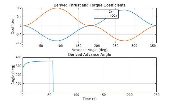
Figure contains 2 axes objects. Axes object 1 with title Derived Thrust and Torque Coefficients, xlabel Advance Angle (deg), ylabel Coefficient contains 2 objects of type line. These objects represent C_T, -10C_Q. Axes object 2 with title Derived Advance Angle, xlabel Time (s), ylabel Angle (deg) contains an object of type line.

The steady-state advance angle is 3 $°$ . Again, the advance angle transitions from the first to forth quadrant, generating positive thrust and torque.

Transient Wind Velocity

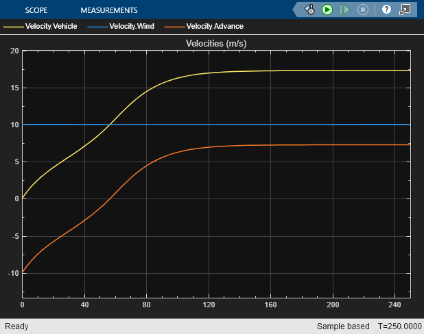
Observe the vehicle dynamics as the wind velocity changes its sign.

set_param("WindPoweredVehicleWithPropeller/Wind Velocity","rep_seq_t","[0 160 165 200 205 250.1]",...
    "rep_seq_y","[10 10 -2 -2 8 8]");                  
sim("WindPoweredVehicleWithPropeller");              
open_system("WindPoweredVehicleWithPropeller/Scope");

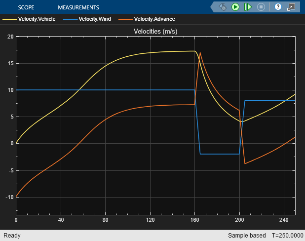
The abrupt change in wind velocity around 160 seconds causes a negative acceleration. The thrust coefficient curves shows that at the increased advance velocity, the advance angle is still in the first quadrant but increases to the point when the thrust coefficient becomes negative. The subsequent change in wind velocity around 200 seconds causes a change in the sign of the advance velocity, leading to the transition from the first quadrant to the fourth quadrant. In the fourth quadrant, the thrust coefficient is positive, causing positive acceleration in the vehicle.