Analyze Tradeoffs Between Performance and Fidelity
Designing physical system models involves balancing model performance and fidelity
compared to a real system. Increasing the fidelity of your model yields more
accurate results but also increases the computational requirements. Applications
such as hardware-in-the-loop (HIL) simulation have strict computational cost
requirements. For these applications, many blocks have parameterizations with the
phrase Suitable for HIL Simulation. These parameterizations use
abstractions to reduce computational cost and increase speed. You can also improve
performance by omitting some physics or lumping parameters. When you adjust fidelity
to improve performance, verify that the updated model results are acceptable
compared to the baseline.
Lower fidelity models prioritize computational efficiency, which allows for faster simulation times and more seamless integration with hardware systems. High-fidelity models use more computational resources to capture physical detail with more accurate results. High-fidelity models may not be suitable for HIL because they require more resources than the target hardware has. For HIL, your specific computational cost requirements depend on your target hardware.
Simplify a Model for Better Performance
You can make a model run faster by avoiding elements that cause discontinuities or fast dynamics. Elements such as hard stops or backlash, stick-slip friction, and clutches are prone to discontinuities. Small masses connected to stiff springs without sufficient damping can cause fast system dynamics that increase the computation cost for a time step.
To see a model that you can configure for performance or high-fidelity, open the Vehicle with Four-Wheel Drive model. Enter:
openExample('sdl/VehicleWithFourWheelDriveExample')Engine, to provide torque to the system. The
Torque Converter block acts as a damper
between the engine and the Simple Gear block
labeled Gearbox. The Gearbox block
transfers torque to both Differential blocks. The
four tire blocks convert the rotational energy into translational energy to
propel the Vehicle Body block, which calculates
the interactions between the tires and the road surface.

The four tire blocks are Variant Subsystem blocks that contain
three tire variants. Each variant uses a different block to represent the tire
dynamics. Double-click the Left Front subsystem to see the
active and inactive variants. To learn more, see Variant Subsystem, Variant Model,
Variant Assembly Subsystem.
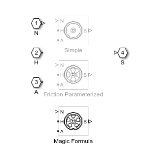
The inactive variants are light gray on the canvas. You can double-click any variant to see the implementations.
The default implementation uses the Tire (Magic
Formula) block, which calculates the tire using slip angle,
longitudinal slip, and vertical load. This block results in high-fidelity
calculations, but the model runs slower to simulate than the other two
implementations. The Simple subsystem uses the
Tire (Simple) block, which represents a
simple no-slip model. Using this subsystem results in a faster model and lower
fidelity tire calculations.
Return to the top level of the model canvas. To enable the
Simple variant on all four tires, click the
Simple hyperlink in bullet 2 of the example links or enter:
VehicleWithFourWheelDriveSetTires(bdroot,'simple')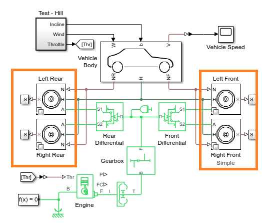
Now all four tires use the Simple parameterization. To
confirm that the Gearbox, Front
Differential, and Rear Differential blocks are
configured for speed, check that Friction model is
No meshing losses - Suitable for HIL Simulation.
Also confirm that Enable backlash is cleared for the
Simple Gear block. The model is now less
complex and can run faster than the default model.
To run the faster model to collect data and plot the time step information, enter:
sim('VehicleWithFourWheelDrive')
simlogRef = simlog_VehicleWithFourWheelDrive;
tireRefNode = simlogRef.Left_Rear.Simple.Tire_Simple.A.w;
tRef = tireRefNode.series.time;
semilogy(tRef(1:end-1),diff(tRef),'-x')
title('Solver Step Size')
xlabel('Time (s)')
ylabel('Step Size (s)')
legend('Simple Tire',location='best')
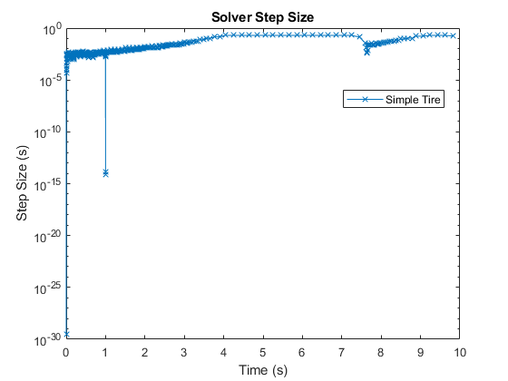
The spike that occurs one second into the simulation indicates that an event caused the solver to take a smaller time step.
Visualize the Difference Between Performance and Fidelity
Now that you have baseline results using a simple implementation of the model, you can analyze the performance cost or benefit of changing model fidelity. Switch the tire variants back to the Tire (Magic Formula) block, run the simulation, and plot the results.
VehicleWithFourWheelDriveSetTires(bdroot,'MFormula')
sim('VehicleWithFourWheelDrive')
simlogRef = simlog_VehicleWithFourWheelDrive;
tireRefNode = simlogRef.Left_Rear.Magic_Formula.Tire_Magic_Formula.A.w;
tRef = tireRefNode.series.time;
hold on
semilogy(tRef(1:end-1),diff(tRef),'-o')
legend('Simple Tire','Magic Formula Tire',location='best')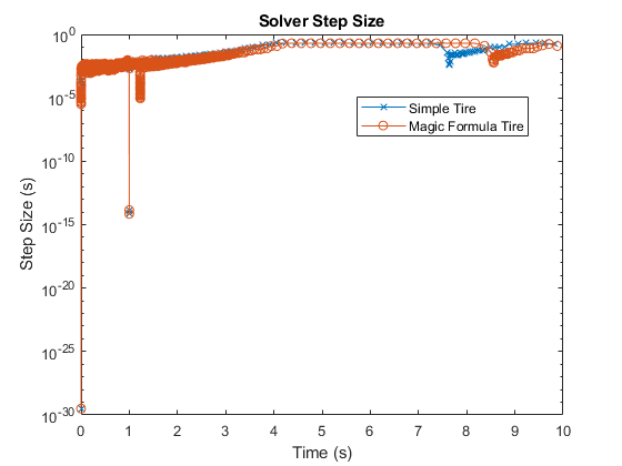
The Magic Formula parameterization is high-fidelity. The denser grouping of time steps at the beginning of the simulation indicates that the model takes longer to initialize. After the first spike at one second into the simulation, the solver reaches a second spike with a slow recovery. Compared to the simple tire parameterization, the solver takes extra resources to compute the results. The smaller step sizes are the result of capturing additional physical behavior in the simulation. The high-fidelity implementation captured an event at approximately 1.2 seconds that the simple tire implementation did not. Zoom in on the results to get a better view.

Also, at approximately eight seconds, the high-fidelity implementation shows an event that occurs later than in the simple implementation.

The high-fidelity model captures more detailed and more accurate results but takes longer to simulate and takes smaller solver steps. You can gain more detailed insights about the simulation by using the Solver Profiler. To learn more about solver step size and real-time model preparation, see Define Step Size and Number of Nonlinear Iterations for Simscape Real-Time Simulation.
See Also
Reduce Zero Crossings | Examine Model Dynamics Using Solver Profiler