Robustness Analysis in Simulink
This example shows how to use Simulink® blocks and helper functions provided by Robust Control Toolbox™ to specify and analyze uncertain systems in Simulink and how to use these tools to perform Monte Carlo simulations of uncertain systems.
Introduction
The Simulink model usim_model consists of an uncertain plant in feedback with a sensor:
open_system('usim_model')
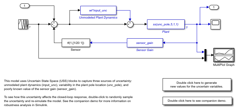
The plant is a first-order model with two sources of uncertainty:
Real pole whose location varies between -10 and -4
Unmodeled dynamics which amount to 25% relative uncertainty at low frequency rising to 100% uncertainty at 130 rad/s.
The feedback path has a cheap sensor which is modeled by a first-order filter at 20 rad/s and an uncertain gain ranging between 0.1 and 2. To specify these uncertain variables, type
% First-order plant model
unc_pole = ureal('unc_pole',-5,'Range',[-10 -4]);
plant = ss(unc_pole,5,1,1);

% Unmodeled plant dynamics
input_unc = ultidyn('input_unc',[1 1]);
wt = makeweight(0.25,130,2.5);

% Sensor gain
sensor_gain = ureal('sensor_gain',1,'Range',[0.1 2]);
Simulink Blocks for Uncertainty Modeling and Analysis
The RCTblocks library contains blocks to model and analyze uncertainty effects in Simulink. To open the library, type
open('RCTblocks')
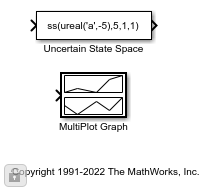
The Uncertain State Space block lets you specify uncertain linear systems (USS objects). usim_model contains three such blocks which are highlighted in blue. The dialog for the "Plant" block appears below.
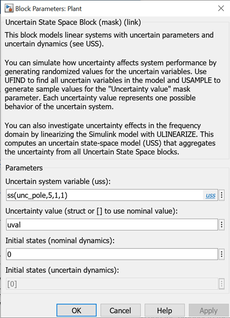
In this dialog box,
The "Uncertain system variable" parameter specifies the uncertain plant model (first-order model with uncertain pole
unc_pole).The "Uncertainty value" parameter specifies values for the block's uncertain variables (
unc_polein this case).
uval is a structure whose field names and values are the uncertain variable names and values to use for simulation. You can set uval to [] to use nominal values for the uncertain variables or vary uval to analyze how uncertainty affects the model responses.
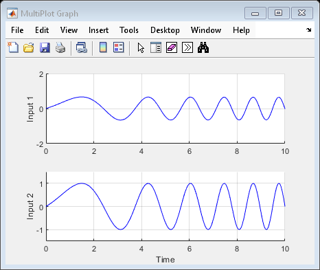
The MultiPlot Graph block is a convenient way to visualize the response spread as you vary the uncertainty. This block superposes the simulation results obtained for each uncertainty value.
Monte Carlo Simulation of Uncertain Systems
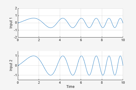
To easily control the uncertainty value used for simulation, usim_model uses the same "Uncertainty value" uval in all three Uncertain State Space blocks. Setting uval to [] simulates the closed-loop response for the nominal values of unc_pole, input_unc, and sensor_gain:
uval = [];   % use nominal value of uncertain variables
sim('usim_model',10);   % simulate response
To analyze how uncertainty affects the model responses, you can use the ufind and usample commands to generate random values of unc_pole, input_unc, and sensor_gain. First use ufind to find the Uncertain State Space blocks in usim_model and compile a list of all uncertain variables in these blocks:
[uvars,pathinfo] = ufind('usim_model');
uvars          % uncertain variables
uvars =

  struct with fields:

      input_unc: [1x1 ultidyn]
    sensor_gain: [1x1 ureal]
       unc_pole: [1x1 ureal]
pathinfo(:,1) % paths to USS blocks
ans =

  3x1 cell array

    {'usim_model/Plant'                   }
    {'usim_model/Sensor Gain'             }
    {'usim_model/Unmodeled Plant Dynamics'}
Then use usample to generate uncertainty values uval consistent with the specified uncertainty ranges. For example, you can simulate the closed-loop response for 10 random values of unc_pole, input_unc, and sensor_gain as follows:
for i=1:10;
   uval = usample(uvars);   % generate random instance of uncertain variables
   sim('usim_model',10);   % simulate response
end
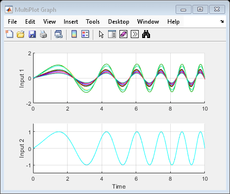
The MultiPlot Graph window now shows 10 possible responses of the uncertain feedback loop. Note that each uval instance is a structure containing values for the uncertain variables input_unc, sensor_gain, and unc_pole:
uval % sample value of uncertain variables
uval =

  struct with fields:

      input_unc: [1x1 ss]
    sensor_gain: 0.5893
       unc_pole: -4.9557
Randomized Simulations
If needed, you can configure the model to use a different uncertainty value uval for each new simulation. To do this, add uvars to the Base or Model workspace and attach the usample call to the model InitFcn:
bdclose('usim_model'), open_system('usim_model')
% Write the uncertain variable list in the Base Workspace
evalin('base','uvars=ufind(''usim_model'');')
% Modify the model InitFcn
set_param('usim_model','InitFcn','uval = usample(uvars);');

% Simulate ten times (same as pressing "Start simulation" ten times)
for i=1:10;
   sim('usim_model',10);
end

% Clean up
set_param('usim_model','InitFcn','');
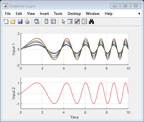
Again the MultiPlot Graph window shows 10 possible responses of the uncertain feedback loop.
Linearization of Uncertain Simulink Models
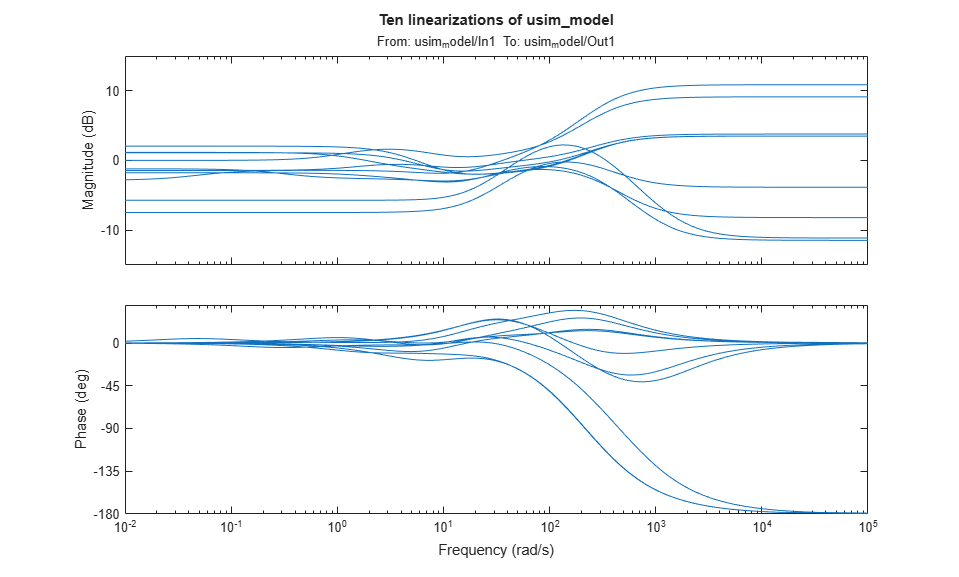
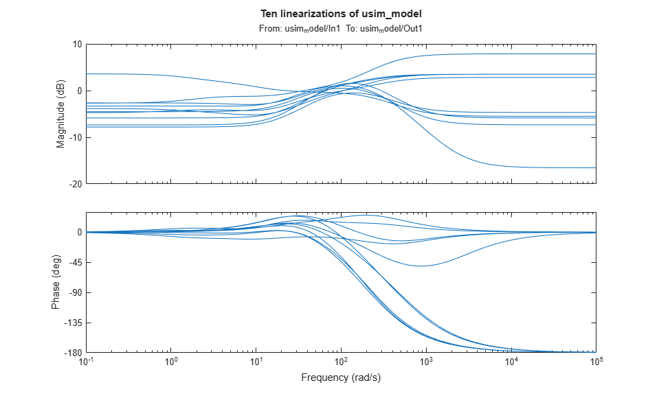
If you have Simulink Control Design™, you can use the same workflow to linearize and analyze uncertain systems in the frequency domain. For example, you can plot the closed-loop Bode response for 10 random samples of the model uncertainty:
clear sys
wmax = 50;  % max natural frequency for unmodeled dynamics (input_unc)
for i=1:10;
   uval = usample(uvars,1,wmax);
   sys(:,:,i) = linearize('usim_model');
end

bode(sys)
title('Ten linearizations of usim\_model');

If the operating point is independent of the uncertain variables, a faster approach is to compute an uncertain linearization (USS object) in one shot using the ulinearize command:
usys = ulinearize('usim_model')
Uncertain continuous-time state-space model with 1 outputs, 1 inputs, 3 states.
The model uncertainty consists of the following blocks:
  input_unc: Uncertain 1x1 LTI, peak gain = 1, 1 occurrences
  sensor_gain: Uncertain real, nominal = 1, range = [0.1,2], 1 occurrences
  unc_pole: Uncertain real, nominal = -5, range = [-10,-4], 1 occurrences

Type "usys.NominalValue" to see the nominal value and "usys.Uncertainty" to interact with the uncertain elements.

You can then sample the uncertain state-space model usys to generate a similar Bode plot:
bode(usample(usys,10,wmax))
title('Ten linearizations of usim\_model');
See Also
Blocks
Functions
Related Topics
You can also select a web site from the following list:
Americas
- América Latina (Español)
- Canada (English)
- United States (English)
Europe
- Belgium (English)
- Denmark (English)
- Deutschland (Deutsch)
- España (Español)
- Finland (English)
- France (Français)
- Ireland (English)
- Italia (Italiano)
- Luxembourg (English)
- Netherlands (English)
- Norway (English)
- Österreich (Deutsch)
- Portugal (English)
- Sweden (English)
- Switzerland
- United Kingdom (English)