modelDiscrimination
Syntax
Description
DiscMeasure = modelDiscrimination(eadModel,data)modelDiscrimination supports segmentation and comparison
against a reference model and alternative methods to discretize the EAD response
into a binary variable.
[
specifies options using one or more name-value arguments in addition to the input
arguments in the previous syntax.DiscMeasure,DiscData] = modelDiscrimination(___,Name=Value)
Examples
This example shows how to use fitEADModel to create a Tobit model and then use modelDiscrimination to compute AUROC and ROC.
Load EAD Data
Load the EAD data.
load EADData.mat
head(EADData)
UtilizationRate Age Marriage Limit Drawn EAD
_______________ ___ ___________ __________ __________ __________
0.24359 25 not married 44776 10907 44740
0.96946 44 not married 2.1405e+05 2.0751e+05 40678
0 40 married 1.6581e+05 0 1.6567e+05
0.53242 38 not married 1.7375e+05 92506 1593.5
0.2583 30 not married 26258 6782.5 54.175
0.17039 54 married 1.7357e+05 29575 576.69
0.18586 27 not married 19590 3641 998.49
0.85372 42 not married 2.0712e+05 1.7682e+05 1.6454e+05
rng('default');
NumObs = height(EADData);
c = cvpartition(NumObs,'HoldOut',0.4);
TrainingInd = training(c);
TestInd = test(c);
Select Model Type
Select a model type for Tobit or Regression.
ModelType =  "Tobit";
Select Conversion Measure
Select a conversion measure for the EAD response values.
ConversionMeasure =  "LCF";
Create Tobit EAD Model
Use fitEADModel to create a Tobit model using the TrainingInd data.
eadModel = fitEADModel(EADData(TrainingInd,:),ModelType,PredictorVars={'UtilizationRate','Age','Marriage'}, ...
    ConversionMeasure=ConversionMeasure,DrawnVar="Drawn",LimitVar="Limit",ResponseVar="EAD");
disp(eadModel);
Tobit with properties:
CensoringSide: "both"
LeftLimit: 0
RightLimit: 1
ModelID: "Tobit"
Description: ""
UnderlyingModel: [1×1 risk.internal.credit.TobitModel]
PredictorVars: ["UtilizationRate" "Age" "Marriage"]
ResponseVar: "EAD"
LimitVar: "Limit"
DrawnVar: "Drawn"
ConversionMeasure: "lcf"
Display the underlying model. The underlying model's response variable is the transformation of the EAD response data. Use the 'LiimitVar' and 'DrwanVar' name-value arguments to modify the transformation.
disp(eadModel.UnderlyingModel);
Tobit regression model:
     EAD_lcf = max(0,min(Y*,1))
     Y* ~ 1 + UtilizationRate + Age + Marriage

Estimated coefficients:
                             Estimate        SE         tStat        pValue
                            __________    _________    ________    __________

    (Intercept)                0.22467     0.030742      7.3083    3.5727e-13
    UtilizationRate             0.4714     0.020845      22.615             0
    Age                     -0.0014209    0.0007528     -1.8875        0.0592
    Marriage_not married     -0.010543     0.015758    -0.66905       0.50353
    (Sigma)                     0.3618    0.0050032      72.314             0

Number of observations: 2627
Number of left-censored observations: 0
Number of uncensored observations: 2626
Number of right-censored observations: 1
Log-likelihood: -1057.9
Predict EAD
EAD prediction operates on the underlying compact statistical model and then transforms the predicted values back to the EAD scale. You can specify the predict function with different options for the 'ModelLevel' name-value argument.
predictedEAD = predict(eadModel,EADData(TestInd,:),ModelLevel="ead");
predictedConversion = predict(eadModel,EADData(TestInd,:),ModelLevel="ConversionMeasure");
Validate EAD Model
For model validation, use modelDiscrimination, modelDiscriminationPlot, modelCalibration, and modelCalibrationPlot.
Use modelDiscrimination and then modelDiscriminationPlot to plot the ROC curve.
ModelLevel = "ConversionMeasure";

[DiscMeasure1,DiscData1] = modelDiscrimination(eadModel,EADData(TestInd,:),ShowDetails=true,ModelLevel=ModelLevel)
"ConversionMeasure";
[DiscMeasure1,DiscData1] = modelDiscrimination(eadModel,EADData(TestInd,:),ShowDetails=true,ModelLevel=ModelLevel)DiscMeasure1=1×3 table
AUROC Segment SegmentCount
_______ __________ ____________
Tobit 0.70893 "all_data" 1751
DiscData1=1534×3 table
        X             Y           T
    __________    _________    _______

             0            0    0.63602
             0    0.0027778    0.63602
             0    0.0041667     0.6349
    0.00096993    0.0055556    0.63377
    0.00096993    0.0069444    0.63265
     0.0019399    0.0083333    0.63152
     0.0029098    0.0097222     0.6304
     0.0029098     0.015278    0.62927
     0.0029098     0.016667    0.62922
     0.0029098     0.018056     0.6288
     0.0029098     0.019444    0.62864
     0.0038797     0.022222    0.62814
     0.0038797        0.025    0.62767
     0.0048497     0.026389    0.62701
     0.0048497     0.033333    0.62654
     0.0058196     0.033333    0.62618
      ⋮
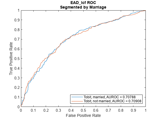
modelDiscriminationPlot(eadModel,EADData(TestInd,:),ModelLevel=ModelLevel,SegmentBy="Marriage");
This example shows how to use fitEADModel to create a Beta model and then use modelDiscrimination to compute AUROC and ROC.
Load EAD Data
Load the EAD data.
load EADData.mat
head(EADData)
UtilizationRate Age Marriage Limit Drawn EAD
_______________ ___ ___________ __________ __________ __________
0.24359 25 not married 44776 10907 44740
0.96946 44 not married 2.1405e+05 2.0751e+05 40678
0 40 married 1.6581e+05 0 1.6567e+05
0.53242 38 not married 1.7375e+05 92506 1593.5
0.2583 30 not married 26258 6782.5 54.175
0.17039 54 married 1.7357e+05 29575 576.69
0.18586 27 not married 19590 3641 998.49
0.85372 42 not married 2.0712e+05 1.7682e+05 1.6454e+05
rng('default');
NumObs = height(EADData);
c = cvpartition(NumObs,'HoldOut',0.4);
TrainingInd = training(c);
TestInd = test(c);
Select Model Type
Select a model type for a Beta model.
ModelType =  "Beta";
Select Conversion Measure
Select a conversion measure for the EAD response values.
ConversionMeasure =  "LCF";
Create Beta EAD Model
Use fitEADModel to create a Beta model using the TrainingInd data.
eadModel = fitEADModel(EADData(TrainingInd,:),ModelType,PredictorVars={'UtilizationRate','Age','Marriage'}, ...
    ConversionMeasure=ConversionMeasure,DrawnVar="Drawn",LimitVar="Limit",ResponseVar="EAD");
disp(eadModel);
Beta with properties:
BoundaryTolerance: 1.0000e-07
ModelID: "Beta"
Description: ""
UnderlyingModel: [1×1 risk.internal.credit.BetaModel]
PredictorVars: ["UtilizationRate" "Age" "Marriage"]
ResponseVar: "EAD"
LimitVar: "Limit"
DrawnVar: "Drawn"
ConversionMeasure: "lcf"
Display the underlying model. The underlying model's response variable is the transformation of the EAD response data. Use the 'LiimitVar' and 'DrwanVar' name-value arguments to modify the transformation.
disp(eadModel.UnderlyingModel);
Beta regression model:
     logit(EAD_lcf) ~ 1_mu + UtilizationRate_mu + Age_mu + Marriage_mu
     log(EAD_lcf) ~ 1_phi + UtilizationRate_phi + Age_phi + Marriage_phi

Estimated coefficients:
                                 Estimate        SE         tStat        pValue
                                __________    _________    ________    __________

    (Intercept)_mu                -0.65566      0.11484     -5.7093    1.2616e-08
    UtilizationRate_mu              1.7014     0.078094      21.787             0
    Age_mu                      -0.0055901    0.0027603     -2.0252      0.042949
    Marriage_not married_mu      -0.012577     0.052098     -0.2414       0.80926
    (Intercept)_phi               -0.50131     0.094625     -5.2979    1.2687e-07
    UtilizationRate_phi            0.39731     0.066707       5.956    2.9307e-09
    Age_phi                      -0.001167    0.0023161    -0.50388       0.61439
    Marriage_not married_phi     -0.013276     0.042627    -0.31144       0.75549

Number of observations: 2627
Log-likelihood: -3140.21
Predict EAD
EAD prediction operates on the underlying compact statistical model and then transforms the predicted values back to the EAD scale. You can specify the predict function with different options for the 'ModelLevel' name-value argument.
predictedEAD = predict(eadModel,EADData(TestInd,:),ModelLevel="ead");
predictedConversion = predict(eadModel,EADData(TestInd,:),ModelLevel="ConversionMeasure");
Validate EAD Model
For model validation, use modelDiscrimination, modelDiscriminationPlot, modelCalibration, and modelCalibrationPlot.
Use modelDiscrimination and then modelDiscriminationPlot to plot the ROC curve.
ModelLevel = "ConversionMeasure";

[DiscMeasure1,DiscData1] = modelDiscrimination(eadModel,EADData(TestInd,:),ShowDetails=true,ModelLevel=ModelLevel)
"ConversionMeasure";
[DiscMeasure1,DiscData1] = modelDiscrimination(eadModel,EADData(TestInd,:),ShowDetails=true,ModelLevel=ModelLevel)DiscMeasure1=1×3 table
AUROC Segment SegmentCount
_______ __________ ____________
Beta 0.70895 "all_data" 1751
DiscData1=1534×3 table
        X             Y           T
    __________    _________    _______

             0            0    0.71675
             0    0.0027778    0.71675
             0    0.0041667    0.71561
             0    0.0055556    0.71533
    0.00096993    0.0069444    0.71447
    0.00096993    0.0097222    0.71419
    0.00096993     0.011111    0.71333
    0.00096993     0.018056    0.71304
     0.0019399     0.018056     0.7128
     0.0029098     0.019444    0.71218
     0.0048497     0.019444     0.7119
     0.0058196     0.020833    0.71104
     0.0067895     0.020833    0.71075
     0.0067895     0.022222    0.71022
     0.0067895     0.027778    0.70989
     0.0067895     0.029167    0.70968
      ⋮
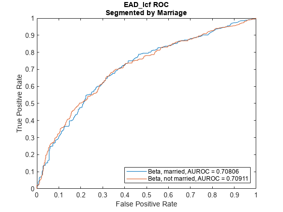
modelDiscriminationPlot(eadModel,EADData(TestInd, :),ModelLevel=ModelLevel,SegmentBy="Marriage");
Input Arguments
Exposure at default model, specified as a previously created Regression,
Tobit, or Beta object using
fitEADModel.
Data Types: object
Data, specified as a
NumRows-by-NumCols table with
predictor and response values. The variable names and data types must be
consistent with the underlying model.
Data Types: table
Name-Value Arguments
Specify optional pairs of arguments as
Name1=Value1,...,NameN=ValueN, where Name is
the argument name and Value is the corresponding value.
Name-value arguments must appear after other arguments, but the order of the
pairs does not matter.
Example: [DiscMeasure,DiscData] =
modelDiscrimination(eadModel,data(TestInd,:),DataID='Testing',DiscretizeBy='median')
Data set identifier, specified as DataID and a
character vector or string. The DataID is included in
the output for reporting purposes.
Data Types: char | string
Discretization method for EAD data at the defined
ModelLevel, specified as
DiscretizeBy and a character vector or string.
'mean'— Discretized response is1if observed EAD is greater than or equal to the mean EAD,0otherwise.'median'— Discretized response is1if observed EAD is greater than or equal to the median EAD,0otherwise.
Data Types: char | string
Name of a column in the data input, not
necessarily a model variable, to be used to segment the data set,
specified as SegmentBy and a character vector or
string. One AUROC is reported for each segment, and the corresponding
ROC data for each segment is returned in the optional output.
Data Types: char | string
Since R2022a
Indicates if the output includes columns showing segment value and
segment count, specified as the comma-separated pair consisting of
'ShowDetails' and a scalar logical.
Data Types: logical
Model level, specified as ModelLevel and a
character vector or string.
Note
Regression models support all three model levels,
but a Tobit
or Beta
model supports only a ModelLevel for
"ead" and
"conversionMeasure".
Data Types: char | string
Identifier for the reference model, specified as
ReferenceID and a character vector or string.
'ReferenceID' is used in the
modelDiscrimination output for reporting
purposes.
Data Types: char | string
Output Arguments
AUROC information for each model and each segment, returned as a table.
DiscMeasure has a single column named
'AUROC' and the number of rows depends on the number
of segments and whether you use a ReferenceID for a
reference model. The row names of DiscMeasure report the
model IDs, segment, and data ID. If the optional
ShowDetails name-value argument is
true, the DiscMeasure output
displays Segment and SegmentCount columns.
Note
If you do not specify SegmentBy and use
ShowDetails to request the segment details,
the two columns are added and show the Segment
column as "all_data" and the sample size (minus
missing values) for the SegmentCount
column.
ROC data for each model and each segment, returned as a table. There are
three columns for the ROC data, with column names 'X',
'Y', and 'T', where the first two
are the X and Y coordinates of the ROC curve, and T contains the
corresponding thresholds. For more information, see Model Discrimination or perfcurve.
If you use SegmentBy, the function stacks the ROC
data for all segments and DiscData has a column with the
segmentation values to indicate where each segment starts and ends.
If reference model data is given, the DiscData outputs
for the main and reference models are stacked, with an extra column
'ModelID' indicating where each model starts and
ends.
More About
Model discrimination measures the risk ranking.
The modelDiscrimination function computes the area under the
receiver operator characteristic (AUROC) curve, sometimes called simply the area
under the curve (AUC). This metric is between 0 and 1 and higher values indicate
better discrimination.
To compute the AUROC, you need a numeric prediction and a binary response. For EAD
models, the predicted EAD is used directly as the prediction. However, the observed
EAD must be discretized into a binary variable. By default, observed EAD values
greater than or equal to the mean observed EAD are assigned a value of 1, and values
below the mean are assigned a value of 0. This discretized response is interpreted
as "high EAD" vs. "low EAD." Therefore, the modelDiscrimination
function measures how well the predicted EAD separates the "high EAD" vs. the "low
EAD" observations. You can change the level to compute the model discrimination with
the ModelLevel name-value pair argument and the discretization
criterion with the DiscretizeBy name-value pair
argument.
To plot the receiver operator characteristic (ROC) curve, use the modelDiscriminationPlot function. However, if you need the ROC curve
data, use the optional DiscData output argument from the
modelDiscrimination function.
The ROC curve is a parametric curve that plots the proportion of
High EAD cases with predicted EAD greater than or equal to a parameter t, or true positive rate (TPR)
Low EAD cases with predicted EAD greater than or equal to the same parameter t, or false positive rate (FPR)
The parameter t sweeps through all the observed predicted EAD
values for the given data. The DiscData optional output
contains the TPR in the 'X' column, the FPR in the
'Y' column, and the corresponding parameters
t in the 'T' column. For more information
about ROC curves, see ROC Curve and Performance Metrics.
References
[1] Baesens, Bart, Daniel Roesch, and Harald Scheule. Credit Risk Analytics: Measurement Techniques, Applications, and Examples in SAS. Wiley, 2016.
[2] Bellini, Tiziano. IFRS 9 and CECL Credit Risk Modelling and Validation: A Practical Guide with Examples Worked in R and SAS. San Diego, CA: Elsevier, 2019.
[3] Brown, Iain. Developing Credit Risk Models Using SAS Enterprise Miner and SAS/STAT: Theory and Applications. SAS Institute, 2014.
[4] Roesch, Daniel and Harald Scheule. Deep Credit Risk. Independently published, 2020.
Version History
Introduced in R2021bThe eadModel input supports an option for a
Beta model object that you can create using fitEADModel.
There is an additional name-value pair for ShowDetails to
indicate if the DiscMeasure output includes columns for
Segment value and the SegmentCount.
MATLAB Command
You clicked a link that corresponds to this MATLAB command:
Run the command by entering it in the MATLAB Command Window. Web browsers do not support MATLAB commands.
Web サイトの選択
Web サイトを選択すると、翻訳されたコンテンツにアクセスし、地域のイベントやサービスを確認できます。現在の位置情報に基づき、次のサイトの選択を推奨します:
また、以下のリストから Web サイトを選択することもできます。
最適なサイトパフォーマンスの取得方法
中国のサイト (中国語または英語) を選択することで、最適なサイトパフォーマンスが得られます。その他の国の MathWorks のサイトは、お客様の地域からのアクセスが最適化されていません。
南北アメリカ
- América Latina (Español)
- Canada (English)
- United States (English)
ヨーロッパ
- Belgium (English)
- Denmark (English)
- Deutschland (Deutsch)
- España (Español)
- Finland (English)
- France (Français)
- Ireland (English)
- Italia (Italiano)
- Luxembourg (English)
- Netherlands (English)
- Norway (English)
- Österreich (Deutsch)
- Portugal (English)
- Sweden (English)
- Switzerland
- United Kingdom (English)