Battery Cycle Life Prediction from Initial Operation Data

This example shows how to predict the remaining cycle life of a fast charging Li-ion battery using linear regression, a supervised machine learning algorithm. Lithium-ion battery cycle life prediction using a physics-based modelling approach is very complex due to varying operating conditions and significant device variability even with batteries from the same manufacturer. For this scenario, machine learning based approaches provide promising results when sufficient test data is available. Accurate battery cycle life prediction at the early stages of battery life would allow for rapid validation of new manufacturing processes. It also allows end-users to identify deteriorated performance with sufficient lead-time to replace faulty batteries. To this end, only the first 100 cycles based features are considered for predicting remaining cycle life and the prediction error is shown to be about 10% [1].

Dataset

The dataset contains measurements from 124 lithium-ion cells with nominal capacity of 1.1 Ah and a nominal voltage of 3.3 V under various charge and discharge profiles. The full dataset can be accessed here [2] with detailed description here [1]. For this example, the data is curated to only contain a subset of measurements relevant to the features being extracted. This reduces the size of the download without changing the performance of the machine learning model being considered. Training data contains measurements from 41 cells, validation data contains measurements from 43 cells and the test data contains measurements from 40 cells. Data for each cell is stored in a structure, which includes the following information:

• Descriptive data: Cell barcode, charging policy, cycle life

• Per-cycle summary data: Cycle number, discharge capacity, internal resistance, charge time

• Data collected within a cycle: Time, temperature, linearly interpolated discharge capacity, linearly interpolated voltage

Load the data from the MathWorks supportfiles site (this is a large dataset, ~1.7GB).

url = 'https://ssd.mathworks.com/supportfiles/predmaint/batterycyclelifeprediction/v1/batteryDischargeData.zip';
websave('batteryDischargeData.zip',url);
unzip('batteryDischargeData.zip')
load('batteryDischargeData');

Feature Extraction

Discharge capacity is a key feature that can reflect the health of a battery, and its value is indicative of driving range in an electric vehicle. Plot discharge capacity for the first 1,000 cycles of cells in training data to visualize its change across the life of a cell.

figure, hold on;
for i = 1:size(trainData,2)
    if numel(trainData(i).summary.cycle) == numel(unique(trainData(i).summary.cycle))
      plot(trainData(i).summary.cycle, trainData(i).summary.QDischarge);      
    end
end
ylim([0.85,1.1]),xlim([0,1000]);
ylabel('Discharge capacity (Ah)');
xlabel('cycle');

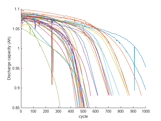
As seen in the plot, capacity fade accelerates near the end of life. However, capacity fade is negligible in the first 100 cycles and by itself is not a good feature for battery cycle life prediction. Therefore, a data-driven approach that considers voltage curves of each cycle, along with additional measurements, including cell internal resistance and temperature, is considered for predicting remaining cycle life. The cycle-to-cycle evolution of Q(V), the discharge voltage curve as a function of voltage for a given cycle, is an important feature space [1]. In particular, the change in discharge voltage curves between cycles, $\Delta Q(V)$, is very effective in degradation diagnosis. Therefore, select the difference in discharge capacity as a function of voltage between 100th and 10th cycle, $$\Delta Q_{100-10}(V)$$.

figure, hold on;
for i = 1:size(testData,2)
    plot((testData(i).cycles(100).Qdlin - testData(i).cycles(10).Qdlin), testData(i).Vdlin)   
end
ylabel('Voltage (V)'); xlabel('Q_{100} - Q_{10} (Ah)');

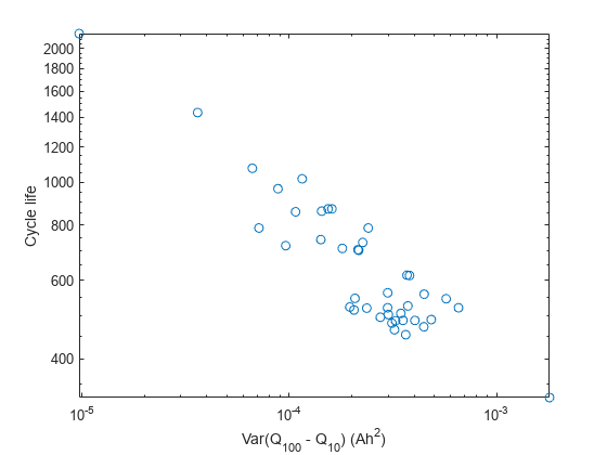
Compute summary statistics using $$\Delta Q_{100-10}(V)$$ curves of each cell as the condition indicator. It is important to bear in mind that these summary statistics do not need to have a clear physical meaning, they just need to exhibit predictive capabilities. For example, the variance of $$\Delta Q_{100-10}(V)$$ and cycle life are highly correlated as seen in this log–log plot, thereby confirming this approach.

figure;
trainDataSize = size(trainData,2);
cycleLife = zeros(trainDataSize,1);
DeltaQ_var = zeros(trainDataSize,1);
for i = 1:trainDataSize
    cycleLife(i) = size(trainData(i).cycles,2) + 1;
    DeltaQ_var(i) = var(trainData(i).cycles(100).Qdlin - trainData(i).cycles(10).Qdlin);
end
loglog(DeltaQ_var,cycleLife, 'o')
ylabel('Cycle life'); xlabel('Var(Q_{100} - Q_{10}) (Ah^2)');

Next, extract the following features from the raw measurement data (the variable names are in brackets) [1]:

• $$\Delta Q_{100-10}(V)$$ log variance [DeltaQ_var]

• $$\Delta Q_{100-10}(V)$$ log minimum [DeltaQ_min]

• Slope of linear fit to capacity fade curve, cycles 2 to 100 [CapFadeCycle2Slope]

• Intercept of linear fit to capacity fade curve, cycles 2 to 100 [CapFadeCycle2Intercept]

• Discharge capacity at cycle 2 [Qd2]

• Average charge time over first 5 cycles [AvgChargeTime]

• Minimum Internal Resistance, cycles 2 to 100 [MinIR]

• Internal Resistance difference between cycles 2 and 100 [IRDiff2And100]

The helperGetFeatures function accepts the raw measurement data and computes the above listed features. It returns XTrain containing the features in a table and yTrain containing the expected remaining cycle life.

[XTrain,yTrain] = helperGetFeatures(trainData);
head(XTrain)

    DeltaQ_var    DeltaQ_min    CapFadeCycle2Slope    CapFadeCycle2Intercept     Qd2      AvgChargeTime     MinIR      IRDiff2And100
    __________    __________    __________________    ______________________    ______    _____________    ________    _____________

     -5.0839       -1.9638          6.4708e-06                1.0809            1.0753       13.409        0.016764     -3.3898e-05 
     -4.3754       -1.6928          1.6313e-05                1.0841            1.0797       12.025        0.016098      4.4186e-05 
     -4.1464       -1.5889          8.1708e-06                  1.08            1.0761       10.968        0.015923     -0.00012443 
     -3.8068       -1.4216          -8.491e-06                1.0974            1.0939       10.025        0.016083     -3.7309e-05 
     -4.1181       -1.6089          2.2859e-05                1.0589            1.0538       11.669        0.015963     -0.00030445 
     -4.0225       -1.5407          2.5969e-05                1.0664            1.0611       10.798        0.016543     -0.00024655 
     -3.9697       -1.5077          1.7886e-05                1.0762            1.0721       10.147        0.016238      2.2163e-05 
     -3.6195       -1.3383         -1.0356e-05                1.0889            1.0851       9.9247        0.016205     -6.6087e-05 

Model Development: Linear Regression with Elastic Net Regularization

Use a regularized linear model to predict the remaining cycle life of a cell. Linear models have low computational cost but provide high interpretability. The linear model is of the form:

$$y_i=w^T{x}_i+\beta$$

where $$y_i$$ is the number of cycles for cell $$i$$, $$x_i$$ is a $$p$$-dimensional feature vector for cell $$i$$ and $$w$$ is $$p$$-dimensional model coefficient vector and $$\beta$$ is a scalar intercept. The linear model is regularized using elastic net to address high correlations between the features. For $$\alpha$$ strictly between 0 and 1, and nonnegative $$\lambda$$, the regularization coefficient, elastic net solves the problem:

$$\underset{}{\overset{ˆ}{w}}={\min }_w\Vert y-Xw-\beta {\Vert }_2^2+\lambda P_{\alpha }(w)$$

where $$P_{\alpha }(w)=\frac{(1-\alpha )}{2}\Vert w{\Vert }_2^2+\alpha \Vert w{\Vert }_1$$. Elastic net approaches ridge regression when $$\alpha$$ is close to 0 and it is the same as lasso regularization when $$\alpha =1$$. Training data is used to choose the hyperparameters $$\alpha$$ and $$\lambda$$, and determine values of the coefficients, $$w$$. The lasso function returns fitted least-squares regression coefficients and information about the fit of the model as output for each $$\alpha$$ and $$\lambda$$ value. The lasso function accepts a vector of values for $$\lambda$$ parameter. Therefore, for each value of $$\alpha$$, the model coefficients $$w$$ and $$\lambda$$ yielding the lowest RMSE value is computed. As proposed in [1], use four-fold cross validation with 1 Monte Carlo repetition for cross-validation.

rng("default")

alphaVec = 0.01:0.1:1;
lambdaVec = 0:0.01:1;
MCReps = 1;
cvFold = 4;

rmseList = zeros(length(alphaVec),1);
minLambdaMSE = zeros(length(alphaVec),1);
wModelList = cell(1,length(alphaVec));
betaVec = cell(1,length(alphaVec));

for i=1:length(alphaVec)
    [coefficients,fitInfo] = ...
        lasso(XTrain.Variables,yTrain,'Alpha',alphaVec(i),'CV',cvFold,'MCReps',MCReps,'Lambda',lambdaVec);
    wModelList{i} = coefficients(:,fitInfo.IndexMinMSE);
    betaVec{i} = fitInfo.Intercept(fitInfo.IndexMinMSE);       
    indexMinMSE = fitInfo.IndexMinMSE;
    rmseList(i) = sqrt(fitInfo.MSE(indexMinMSE));    
    minLambdaMSE(i) = fitInfo.LambdaMinMSE;    
end

To make the fitted model robust, use validation data to select final values of $$\alpha$$ and $$\lambda$$ hyperparameters. To this end, pick the coefficients corresponding to the four lowest RMSE values computed using the training data.

numVal = 4;
[out,idx] = sort(rmseList);
val = out(1:numVal);
index = idx(1:numVal);

alpha = alphaVec(index);
lambda = minLambdaMSE(index);
wModel = wModelList(index);
beta = betaVec(index);

For each set of coefficients, compute the predicted values and RMSE on validation data.

[XVal,yVal] = helperGetFeatures(valData);
rmseValModel = zeros(numVal);
for valList = 1:numVal   
   yPredVal = (XVal.Variables*wModel{valList} + beta{valList});
   rmseValModel(valList) = sqrt(mean((yPredVal-yVal).^2));
end

Select the model with the least RMSE when using the validation data. The model related to the lowest RMSE value for training data is not the model corresponding to the lowest RMSE value for validation data. Using the validation data thereby increases model robustness.

[rmseMinVal,idx] = min(rmseValModel);
wModelFinal = wModel{idx};
betaFinal = beta{idx};

Performance evaluation of the trained model

The test data contains measurements corresponding to 40 cells. Extract the features and the corresponding responses from testData. Use the trained model to predict the remaining cycle life of each cell in testData.

[XTest,yTest] = helperGetFeatures(testData);
yPredTest = (XTest.Variables*wModelFinal + betaFinal);

Visualize the predicted vs. actual cycle life plot for the test data.

figure;
scatter(yTest,yPredTest)
hold on;
refline(1, 0);
title('Predicted vs Actual Cycle Life')
ylabel('Predicted cycle life');
xlabel('Actual cycle life');

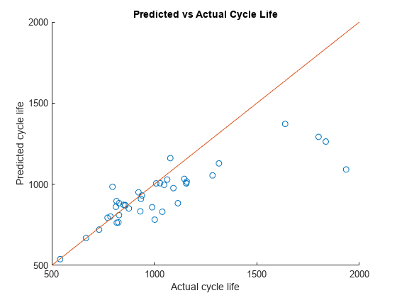
Ideally, all the points in the above plot should be close to the diagonal line. From the above plot, it is seen that the trained model is performing well when the remaining cycle life is between 500 and 1200 cycles. Beyond 1200 cycles, the model performance deteriorates. The model consistently underestimates the remaining cycle life in this region. This is primarily because test and validation data sets contain significantly more cells with total life around 1000 cycles.

Compute the RMSE of the predicted remaining cycle life.

errTest = (yPredTest-yTest);
rmseTestModel = sqrt(mean(errTest.^2))

rmseTestModel = 211.6148

Another metric considered for performance evaluation is average percentage error defined [1] as

$$\%err=\frac{1}{n}{\Sigma }_{i=1}^n\frac{|y_i-{\underset{}{\overset{ˆ}{y}}}_i|}{y_i}\times 100$$

n = numel(yTest);
nr = abs(yTest - yPredTest);
errVal = (1/n)*sum(nr./yTest)*100

errVal = 9.9817

Conclusion

This example showed how to use a linear regression model with elastic net regularization for battery cycle life prediction based on measurements from only the first 100 cycles. Custom features were extracted from the raw measurement data and a linear regression model with elastic net regularization was fitted using training data. The hyperparameters were then selected using the validation dataset. This model was used on test data for performance evaluation. Using measurements for just the first 100 cycles, RMSE of remaining cycle life prediction of cells in the test data set is 211.6 and an average percentage error of 9.98% is obtained.

References

[1] Severson, K.A., Attia, P.M., Jin, N. et al. "Data-driven prediction of battery cycle life before capacity degradation." Nat Energy 4, 383–391 (2019). https://doi.org/10.1038/s41560-019-0356-8

[2] https://data.matr.io/1/

Supporting Functions

function [xTable, y] = helperGetFeatures(batch)
% HELPERGETFEATURES function accepts the raw measurement data and computes
% the following feature:
%
% Q_{100-10}(V) variance [DeltaQ_var]
% Q_{100-10}(V) minimum [DeltaQ_min]
% Slope of linear fit to the capacity fade curve cycles 2 to 100 [CapFadeCycle2Slope]
% Intercept of linear fit to capacity fade curve, cycles 2 to 100 [CapFadeCycle2Intercept]
% Discharge capacity at cycle 2 [Qd2]
% Average charge time over first 5 cycles [AvgChargeTime]
% Minimum Internal Resistance, cycles 2 to 100 [MinIR]
% Internal Resistance difference between cycles 2 and 100 [IRDiff2And100]

N = size(batch,2); % Number of batteries

% Preallocation of variables
y = zeros(N, 1);
DeltaQ_var = zeros(N,1);
DeltaQ_min = zeros(N,1);
CapFadeCycle2Slope = zeros(N,1);
CapFadeCycle2Intercept = zeros(N,1);
Qd2 = zeros(N,1);
AvgChargeTime = zeros(N,1);
IntegralTemp = zeros(N,1);
MinIR = zeros(N,1);
IRDiff2And100 = zeros(N,1);

for i = 1:N
    % cycle life
    y(i,1) = size(batch(i).cycles,2) + 1;
    
    % Identify cycles with time gaps
    numCycles = size(batch(i).cycles, 2);
    timeGapCycleIdx = [];
    jBadCycle = 0;
    for jCycle = 2: numCycles
        dt = diff(batch(i).cycles(jCycle).t);
        if max(dt) > 5*mean(dt)
            jBadCycle = jBadCycle + 1;
            timeGapCycleIdx(jBadCycle) = jCycle;
        end
    end
    
    % Remove cycles with time gaps
    batch(i).cycles(timeGapCycleIdx) = [];
    batch(i).summary.QDischarge(timeGapCycleIdx) = [];
    batch(i).summary.IR(timeGapCycleIdx) = [];
    batch(i).summary.chargetime(timeGapCycleIdx) = [];
    
    % compute Q_100_10 stats
    DeltaQ = batch(i).cycles(100).Qdlin - batch(i).cycles(10).Qdlin;
    DeltaQ_var(i) = log10(abs(var(DeltaQ)));
    DeltaQ_min(i) = log10(abs(min(DeltaQ)));
    
    % Slope and intercept of linear fit for capacity fade curve from cycle
    % 2 to cycle 100
    coeff2 = polyfit(batch(i).summary.cycle(2:100), batch(i).summary.QDischarge(2:100),1);
    CapFadeCycle2Slope(i) = coeff2(1);
    CapFadeCycle2Intercept(i) = coeff2(2);
    
    %  Discharge capacity at cycle 2
    Qd2(i) = batch(i).summary.QDischarge(2);
    
    % Avg charge time, first 5 cycles (2 to 6)
    AvgChargeTime(i) = mean(batch(i).summary.chargetime(2:6));
    
    % Integral of temperature from cycles 2 to 100
    tempIntT = 0;
    for jCycle = 2:100
        tempIntT = tempIntT + trapz(batch(i).cycles(jCycle).t, batch(i).cycles(jCycle).T);
    end
    IntegralTemp(i) = tempIntT;
    
    % Minimum internal resistance, cycles 2 to 100
    temp = batch(i).summary.IR(2:100);
    MinIR(i) = min(temp(temp~=0));
    IRDiff2And100(i) = batch(i).summary.IR(100) - batch(i).summary.IR(2);
end

xTable = table(DeltaQ_var, DeltaQ_min, ...
    CapFadeCycle2Slope, CapFadeCycle2Intercept,...
    Qd2, AvgChargeTime, MinIR, IRDiff2And100);

end