Compute Orientation from Recorded IMU Data
Load the rpy_9axis file into the workspace. The file contains recorded accelerometer, gyroscope, and magnetometer sensor data from a device oscillating in pitch (around the y-axis), then yaw (around the z-axis), and then roll (around the x-axis). The file also contains the sample rate of the recording.
load("rpy_9axis.mat","sensorData")
Read the acceleration and gyroscope readings from the recorded sensor data.
accel = sensorData.Acceleration;
gyro = sensorData.AngularVelocity;
Example Model
Open the Simulink® model.
modelname = "ComputeOrientationFromIMUData";
open_system(modelname)
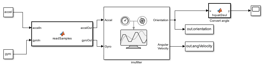
The model reads the accelerometer readings and gyroscope readings from the MATLAB® workspace by using the Constant block. The sample rate of the Constant block is set to the sampling rate of the sensor. In this example, the sample rate is set to 0.005. The model uses the custom MATLAB Function block readSamples to input one sample of sensor data to the IMU Filter block at each simulation time step. Then, the model computes an estimate of the sensor body orientation by using an IMU Filter block with these parameters:
Reference frame —
NEDOrientation format —
quaternionDecimation factor —
1Initial process noise —
imufilter.defaultProcessNoiseAccelerometer noise —
0.0001924722Gyroscope noise —
9.1385e-5Gyroscope drift noise —
3.0462e-13Linear acceleration noise —
0.0096236100000000012Linear acceleration decay factor —
0.5Simulate using —
Interpreted execution
By default, the IMU Filter block outputs the orientation as a vector of quaternions. The model uses the custom MATLAB Function block hquat2eul to convert the quaternion angles to Euler angles.
Simulate Model
Set the start time to 0.005 seconds and the stop time to 8 seconds. You can compute the stop time as  .
.
set_param(modelname,"StartTime","0.005","StopTime","8")
Run the model. The IMU Filter block combines the data from the accelerometer and gyroscope readings and computes the sensor body orientation along the x-, y-, and z-directions. The model then plots the computed results. The model uses the Scope block to plot the computed sensor body orientation over time.
sim(modelname);