predictSNR
Description
[
predicts the signal-to-noise ratio (SNR) versus the input amplitude curve of a binary
delta-sigma modulator using the describing function method [1].snr,amp,k0,k1,sigma_e2] = predictSNR(ntf,osr,amp,f0)
The describing function method assumes that the quantizer processes signal and noise components separately. The method models the quantizer as two linear gains, k0 and k1 and an additive white Gaussian noise source of power sigma_e2. The function assumes nearly infinite gain at the loop filter of the modulator at the test frequency.
Examples
Define a second-order delta-sigma modulator and the system parameters for the simulation.
order = 2;              % The "Order" of the modulator
OSR = 64;               % Oversampling Ratio (fs / 2*BW)
nlev = 2;               % Number of quantizer levels (2 = Binary: +1 or -1)
N = 2^14;               % Number of points for the FFT simulation (16,384)
test_freq = 5;          % The bin index for our test sine wave (must be an integer)
Determine the in-band frequency range for SNR calculation.
fB = floor(N/(2*OSR));
Synthesize the noise transfer function (NTF). This creates a mathematical filter that pushes noise to high frequencies.
ntf = synthesizeNTF(order, OSR);
Realize the NTF as a CIFB circuit topology.
[a, g, b, c] = realizeNTF(ntf, 'CIFB');Create the state-space matrix for the simulator.
abcd = stuffABCD(a, g, b, c, 'CIFB');Scale the ABCD matrix so that the internal voltages stay within the range of the quantizer.
[abcd_scaled, umax] = scaleABCD(abcd, nlev);
To set up the simulation, define a range of input amplitudes to test, from very quiet to loud. Run simulation.
amp_db = -110:10:-10;        % Decibels relative to Full Scale (dBFS)
amp_lin = 10.^(amp_db/20);   % Convert dB to linear voltage
snr_sim = zeros(size(amp_db)); % Pre-allocate space for results
for i = 1:length(amp_db)
    % Generate a test sine wave at the current amplitude
    t = 0:N-1;
    u = amp_lin(i) * sin(2*pi*test_freq/N * t);

    % Run the Delta-Sigma Modulator Simulation
    % Returns 'v', which is the high-speed 1-bit output bitstream.
    v = simulateDSM(u, abcd_scaled, nlev);

    % Spectral Analysis:
    % 1. Apply a Hann window to prevent spectral leakage
    w = ds_hann(N);
    % 2. Perform the FFT
    V = fft(v .* w);
    % 3. Calculate SNR of the in-band portion
    % calculateSNR sums signal power at 'test_freq' and noise in remaining bins.
    snr_sim(i) = calculateSNR(V(1:fB), test_freq);
end
Predict the theoretical SNR. Calculate a peak value to anchor the predicted SNR curve.
peak_snr_theory = 10*log10( ((2*order+1)/(2*pi^(2*order))) * (OSR^(2*order+1)) );
snr_pred = peak_snr_theory + amp_db;
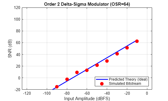
Plot the predicted and simulated SNR.
figure('Color', 'w', 'Name', 'Delta-Sigma Performance');

% Plot the Theoretical Limit (The Blue Line)
plot(amp_db, snr_pred, 'b-', 'LineWidth', 2); hold on;

% Plot the Actual Simulated Results (The Red Dots)
plot(amp_db, snr_sim, 'ro', 'MarkerFaceColor', 'r', 'MarkerSize', 8);

% Formatting the plot
grid on;
axis([-125 5 -20 120]); % Set fixed view for comparison
xlabel('Input Amplitude (dBFS)');
ylabel('SNR (dB)');
title(sprintf('Order %d Delta-Sigma Modulator (OSR=%d)', order, OSR));
legend('Predicted Theory (Ideal)', 'Simulated Bitstream', 'Location', 'SouthEast');
Input Arguments
Output Arguments
References
[1] Ardalan, S., and J. Paulos. “An Analysis of Nonlinear Behavior in Delta - Sigma Modulators.” IEEE Transactions on Circuits and Systems 34, no. 6 (1987): 593–603. https://doi.org/10.1109/TCS.1987.1086187.
Version History
Introduced in R2026a
See Also
calculateTF | synthesizeNTF | realizeNTF | stuffABCD | mapABCD | scaleABCD | calculateSNR | simulateSNR | simulateDSM