Creating a Stewart Platform Model Using SimMechanics
Abstract
SimMechanics, in conjunction with Simulink and MATLAB, enables engineers to model complicated mechanical systems, simulate and analyze the models, and develop controllers for the mechanical system. In this technical example, we examine how to use SimMechanics to model physical components, synthesize controllers, and simulate the closed loop performance of a Stewart Platform, a six degrees-of-freedom positioning system. Stewart Platforms are used in many applications for positioning objects.
Various Applications of the Stewart Platform
The Stewart Platform was originally designed in 1965 as a flight simulator, and it is still commonly used for that purpose. Since then, a wide variety of applications have benefited from this design. A few of the industries using the Stewart Platform design include aerospace and defense, automotive, transportation, and machine tool technology, who use the platform to perform flight simulation, handle vehicle maintenance, and design crane hoist mechanisms. The Stewart Platform design is also used for the positioning of satellite communication dishes and telescopes and in applications such as shipbuilding, bridge construction, transportation, and as a drilling platform on the Lunar Rover.
Specifications of the Stewart Platform
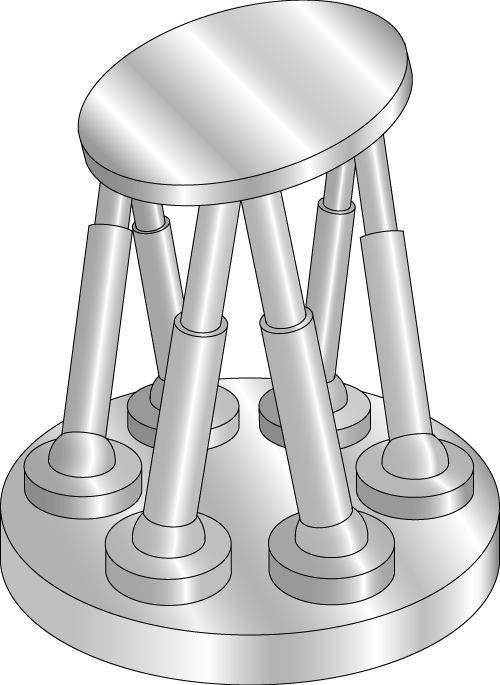
The Stewart Platform is a classic example of a mechanical design that is used for position control. It is a parallel mechanism that consists of a rigid body top plate, or mobile plate, connected to a fixed base plate and is defined by at least three stationary points on the grounded base connected to six independent kinematic legs. Typically, the six legs are connected to both the base plate and the top plate by universal joints in parallel located at both ends of each leg. The legs are designed with an upper body and lower body that can be adjusted, allowing each leg to be varied in length.
The position and orientation of the mobile platform varies depending on the lengths to which the six legs are adjusted. The Stewart Platform can be used to position the platform in six degrees of freedom (three rotational degrees of freedom, as well as three translational degrees of freedom). In general, the top plate is triangularly shaped and is rotated 60 degrees from the bottom plate, allowing all legs to be equidistant from one another and each leg to move independently of the others.
Advantages of the Stewart Platform
Engineers and researchers have examined many variants of the Stewart Platform. Most variants have six linearly actuated legs with varying combinations of leg-platform connections. Of the many types of motion control platforms, the Stewart Platform is useful to study because it is a widely accepted design for a motion control device. This is largely because of the system's wide range of motion and accurate positioning capability. It provides a large amount of rigidity, or stiffness, for a given structural mass, enabling the Stewart Platform system to provide a significant source of positional certainty.
The design of the Stewart Platform supports a high load-carrying capacity. Because of the design, the legs carry compression and tension forces, and will not succumb to the undesirable bending force found in other designs. The six legs are spaced around the top plate and share the load on the top plate. This differs from serial designs, such as robot arms, where the load is supported over a long moment arm.
Defining a Control Problem for the Stewart Platform
The problem addressed in this example is to find a method to actuate the six leg forces to properly position the mobile plate of the Stewart Platform given a desired trajectory. For this particular problem, we are given a desired position and orientation of the mobile plate with respect to the fixed base plate. These desired values might change over time. We wish to control the nonlinear plant model of the Stewart Platform and have inputs and outputs to accomplish this. The six leg forces are the inputs into the plant while the outputs are the lengths and velocities of the six legs. Our task is to create a control strategy and design that will make the top plate follow the desired trajectory. We must accomplish this by actuating the six leg forces, sensing the leg lengths and velocities, and reading the desired trajectory.
Traditionally, a common method for designing the controller for the Stewart Platform required manipulating complicated equations that modeled the physical components used to solve the mechanical equations. Then, the engineer had to solve these equations using complex numerical integration techniques. With the advent of computational tools such as dynamic simulation software, it is now possible to easily model and simulate the Stewart Platform mechanics together with the control system.
Constructing a Stewart Platform Model Using SimMechanics
In this article, we will demonstrate how SimMechanics, Simulink, and MATLAB can be used to model and simulate the behavior of the Stewart Platform. SimMechanics will be used to model the mechanical components of the system, and Simulink will be used to model the controller. Using the predefined libraries from SimMechanics, we will be able to model the Stewart Platform without needing to explicitly derive the equations of motion, which can be a tedious and error-prone process.
Modeling the Physical Components with SimMechanics
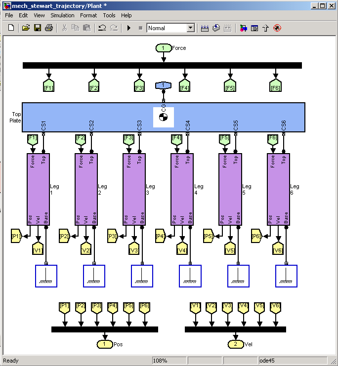
We will first build the plant model using SimMechanics. The mechanical components of the Stewart Platform consist of a top plate, a bottom plate, and six legs connecting the top plate to the bottom plate. The overall system has six degrees of freedom. Each leg subsystem contains two bodies connected together with a cylindrical joint. The upper body connects to the top mobile plate using a universal joint, and the lower body connects to the base plate using a second universal joint.
Using SimMechanics Body blocks, we model the rigid bodies for the base plate, top plate, and upper and lower legs. Next, we connect the bodies together using SimMechanics Joint blocks.
When beginning to build the physical model of the Stewart Platform, we first need to define attachment points relative to an inertial frame (or world). We define this by using a Ground block from the Bodies Library in SimMechanics. The Ground block acts as a fixed point for attaching system components.
Now we will build the legs of the Stewart Platform by connecting the Ground block to the Universal Joint block, and connecting that to a Body block to create the lower leg. Next, we add another Body block to represent the upper leg. Then we use a Cylindrical Joint block to connect the lower leg to the upper leg, enabling the entire leg to adjust its length by moving in one translational and one rotational degree of freedom. Next, we simply add another Universal Joint block connected to the Upper Leg Body block, which will ultimately be attached to the top plate.
Linear actuation of the Stewart Platform is accomplished by varying the lengths of the legs. To move the legs, we use a Joint Actuator block from the Sensor & Actuators Library in SimMechanics. This joint actuator is used to control the translational degree of freedom of the cylindrical joint. (The rotational degree of freedom is unconstrained.) A force signal will be created and used for actuation, rather than using the displacement. This enables us to create a more realistic model of the Stewart Platform where hydraulic actuators can be used to apply force between the upper and lower legs. We are also sensing the length of the leg with a Joint Sensor block from the Sensors & Actuators Library to extract the position and velocity, which will be used by the controller.
By creating a library subsystem of the leg component, we can easily create six instances of the legs of our Stewart Platform model. Now we can connect each of the joints connected to the upper part of each of our six legs to one Body block that will be our top plate. This represents the plant portion of our Stewart Platform model, which will accept inputs of actuation of the top plate as well as the force, position, and velocity signals.
Defining the Geometry Using an M-file Script
Using M-file scripts and custom library blocks is a powerful technique in SimMechanics that enables you to create complicated mechanical models. We demonstrate this technique in this example.
After we have created the physical components of the Stewart Platform model with SimMechanics, we need to define the specific geometry in its initial configuration and the dynamic parameters for the Stewart Platform. These variable definitions will be written in a basic MATLAB script and referenced in the dialog boxes of the blocks that we use to build the SimMechanics model.
First, we define basic angular unit conversions and axes.
deg2rad = pi/180;
x_axis = [1 0 0];
y_axis = [0 1 0];
z_axis = [0 0 1];
Now we define the connection points on the base and top plate with respect to the world frame of reference at the center of the base plate. The definitions below represent the offset angle of 60 degrees between the base and top plate, the radii for both the base and top plate, and the initial position height of the system.
pos_base = [];
pos_top = [];
alpha_b = 2.5*deg2rad;
alpha_t = 10*deg2rad;
height = 2.0;
radius_b = 3.0;
radius_t = 1.0;
for i = 1:3,
% base points
angle_m_b = (2*pi/3)* (i-1) - alpha_b;
angle_p_b = (2*pi/3)* (i-1) + alpha_b;
pos_base(2*i0,:) = radius_b* [cos(angle_m_b), sin(angle_m_b), 0.0];
pos_base(2*i,:) = radius_b* [cos(angle_p_b), sin(angle_p_b), 0.0];
% top points (with a 60 degree offset)
angle_m_t = (2*pi/3)* (i-1) - alpha_t + 2*pi/6;
angle_p_t = (2*pi/3)* (i-1) + alpha_t + 2*pi/6;
pos_top(2*i0,:) = radius_t* [cos(angle_m_t), sin(angle_m_t), height];
pos_top(2*i,:) = radius_t* [cos(angle_p_t), sin(angle_p_t), height];
end
The following permutes the array of the top points so that the index in the top points and the bottom points refers to connection points for a single leg. The points in the top plate coordinate system are defined as well. The leg vectors and unit leg vectors are calculated.
pos_top = [pos_top(6,:); pos_top(1:5,:)];
body_pts = pos_top' - height*[zeros(2,6);ones(1,6)]; legs = pos_top - pos_base;
leg_length = [ ];
leg_vectors = [ ];
for i = 1:6,
leg_length(i) = norm(legs(i,:));
leg_vectors(i,:) = legs(i,:) / leg_length(i);
end
Below is a loop that calculates the revolute and cylindrical axes that will be input into the joint blocks in the physical plant model. There are two revolutes for the Universal Joint block that is connected to the top plate, one cylindrical and one revolute for the linear motion of the Cylindrical Joint block, and two revolutes for the Universal Joint block that is connected to the base plate.
for i = 1:6,
rev1(i,:) = cross(leg_vectors(i,:), z_axis);
rev1(i,:) = rev1(i,:) / norm(rev1(i,:));
rev2(i,:) = - cross(rev1(i,:), leg_vectors(i,:));
rev2(i,:) = rev2(i,:) / norm(rev2(i,:));
cyl1(i,:) = leg_vectors(i,:);
rev3(i,:) = rev1(i,:);
rev4(i,:) = rev2(i,:);
end
Each Body block needs a defined coordinate system for the center of gravity.
lower_leg = struct('origin', [0 0 0], 'rotation', eye(3), 'end_point', [0 0 0]);
upper_leg = struct('origin', [0 0 0], 'rotation', eye(3), 'end_point', [0 0 0]);
for i = 1:6,
lower_leg(i).origin = pos_base(i,:) + (3/8)*legs(i,:);
lower_leg(i).end_point = pos_base(i,:) + (3/4)*legs(i,:);
lower_leg(i).rotation = [rev1(i,:)', rev2(i,:)', cyl1(i,:)'];
upper_leg(i).origin = pos_base(i,:) + (1-3/8)*legs(i,:);
upper_leg(i).end_point = pos_base(i,:) + (1/4)*legs(i,:);
upper_leg(i).rotation = [rev1(i,:)', rev2(i,:)', cyl1(i,:)'];
end
Now we will calculate the inertia and mass for the top plate, bottom plate, and the legs. The density of steel has been used for this calculation:
top_thickness = 0.05;
base_thickness = 0.05;
inner_radius = 0.03;
outer_radius = 0.05;
density = 76e3/9.81; % Kg/m^3
The leg inertia and mass are calculated here in a function called inertiaCylinder, which calculates the mass and inertia of a cylinder given the density, length, and inner and outer radius of the cylinder:
[lower_leg_mass, lower_leg_inertia] = inertiaCylinder(density, ...
     0.75*leg_length(1),outer_radius, inner_radius);
[upper_leg_mass, upper_leg_inertia] = inertiaCylinder(density, ...
     0.75*leg_length(1),inner_radius, 0);
The top and base plate inertia and mass are calculated here using the same function as we used for the legs, accepting inputs of density, plate thickness, and plate radius:
[top_mass, top_inertia] = inertiaCylinder(density, ...
     top_thickness, radius_t, 0);
[base_mass, base_inertia] = inertiaCylinder(density, ...
     base_thickness,radius_b, 0);
Controller Strategy
In typical serial robot applications, the forward kinematics problem is easy while the inverse kinematics problem is more difficult. The forward kinematics problem calculates the position and orientation of the end effector of the robot given the joint angles while the inverse kinematics problem calculates the joint angles (multiple) given the end effector position and orientation. In the Stewart Platform, it is easy to calculate the joint angles (leg lengths) given the position and orientation of the end effector (top plate).
The basic goal of this controller is to specify the desired trajectory of the top plate in both position and orientation. We then map this desired trajectory to the corresponding trajectory in the legs using inverse kinematics. Finally, we use a lower level controller for each leg to command the leg to follow the desired trajectory. In this way, we avoid solving the difficult forward kinematics problem for the Stewart Platform.
The controller consists of two sections: the leg trajectory and the controller. The leg trajectory generates the desired leg lengths for each time step. It starts with a desired rotation and position of the top plate and calculates the desired leg lengths to achieve this. The following equation calculates the leg lengths for each leg:
where R is the rotation matrix relating the top plate orientation with respect to the bottom plate, Pt,i is the attachment point of leg i in the top plate with respect to the top plate coordinate system, P is the position of the top plate with respect to the bottom plate, Pb,i is the attachment point of leg i in the bottom plate with respect to the bottom plate coordinate system, and ln,i is the nominal length of leg i. The leg trajectory subsystem and all of the other blocks in this subsystem implement this equation for each of the six legs.
Simple PID Low-Level Controller
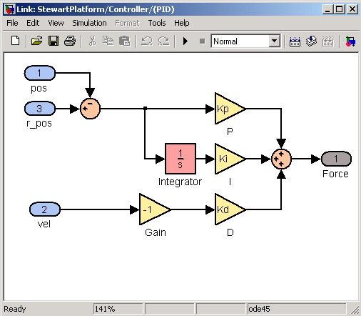
We first implement a simple low-level controller based on the classic PID design. The input to this controller is the actual leg position and velocity and the desired leg position. The leg trajectory subsystem does not generate leg velocities, although a more complicated one could. We then form an error in the position and create a force based on the gain and integral of the error. We also provide a velocity feedback term.
We can develop more sophisticated low-level controllers but we first need to linearize about an equilibrium point.
Linearizing the Model
We now extract a linear model of the Stewart Platform so that we can use more powerful linear control design techniques such as those found in the µ-Analysis and Synthesis Toolbox.
First, we must find the equilibrium point for our nonlinear model. We do this by extracting the equilibrium forces for each leg that keep the Stewart Platform stationary. These are the forces that are being applied when the system is in the initial resting state. To do this, we first extract the plant model into a new Simulink model and then set the Actuator block property to motion and set the position, velocity, and acceleration to zero. We also set the Sensor block for each leg to extract the computed force. To find the equilibrium point where the net force acting on the model is zero, we need to change the Analysis Mode parameter.
In the Simulink model, we select the Mechanical Environment Settings under the Simulation menu. This will display the mechanical parameters that we set for our model. By changing the Analysis Mode, SimMechanics can compute the motion that results from applying forces to a mechanical system or the forces required to produce a specified motion in a mechanical system. Here, the Kinematic Analysis Mode is selected because the Stewart Platform is a closed-loop system, and we want to compute the forces applied without the system moving. Once this is selected, we simulate the model and use the output from the Sensor blocks to obtain the force that will be applied to the Actuator blocks for each of the legs when the platform is at rest. To do this at the MATLAB command prompt, we can use:
sim('StewartPlatformEquilibrium'); u = Forces';
Now, we are ready to extract linear models. To linearize the model near the equilibrium point, we can use the linmod command on just the plant model:
[A,B,C,D] = linmod('StewartPlatformPlant',[],u);
This will generate an LTI state-space model from a SimMechanics model to use as an input to the Control Systems Toolbox and the µ-Analysis and Synthesis Toolbox commands that generate controller models.
The linearization command returns an LTI system with the same number of states as the number of states in the tree of the mechanical system (52 in this case). Since this model is closed, the number of independent states is smaller (12 in this case). We use the minreal function to get at the minimal realization of the plant with 12 states:
[A,B,C,D] = minreal(A,B,C,D);
These are the state-space matrices that we will use to design the controller for the Stewart Platform model.
Designing the Multivariable Controller
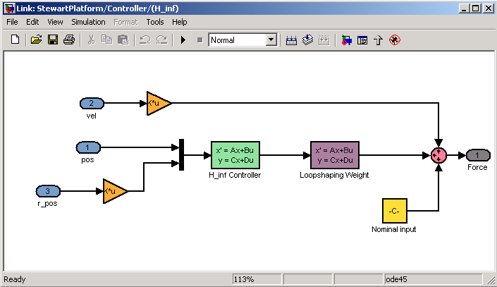
We now use the Control System Toolbox and the µ-Analysis and Synthesis Toolbox to synthesize a multivariable, robust controller for the Stewart Platform. The details of the design, which we don't include here, can be found in the file StewartMVController.m. You can simulate the Stewart Platform with the multivariable controller by changing the controller configurable subsystem to use the H_inf controller.
Simulate and Visualize the Model
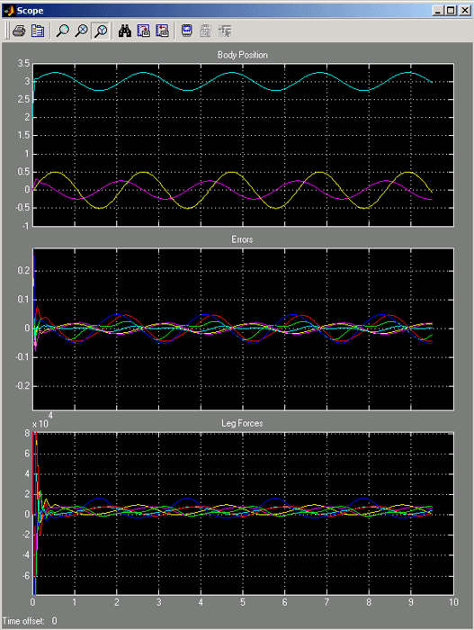
Now that we have modeled our system with Simulink and SimMechanics, we can validate the design by simulating the system. We start the simulation by selecting Simulink and Start in the model window menu bar. During the simulation, we can view signals with the Scope block. The first plot in our scope shows the x, y, and z values of the position of the Body block representing the top plate moving over time as the model simulates. The second plot shows the difference between the desired value of the leg lengths calculated in the Leg Trajectory subsystem and the actual value of the leg lengths changing over time. The third plot shows the force on each leg during the simulation.
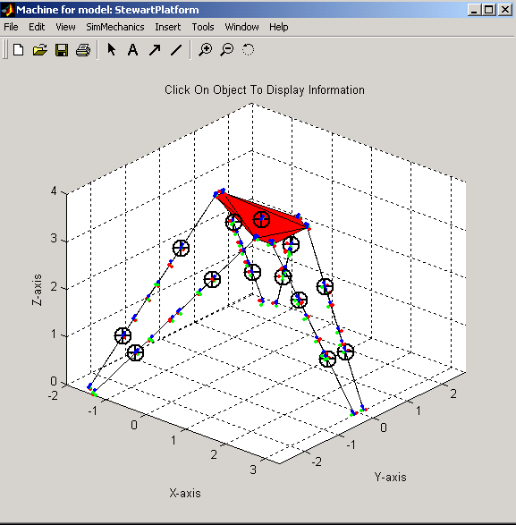
The Virtual Reality Toolbox or MATLAB graphics options can be used to create three-dimensional animations for systems designed in SimMechanics. Either tool can be used to analyze the numerical results that quantify the motion of your mechanical system. Let's view the basic animation provided by MATLAB graphics. The Visualization tab under the Mechanical Environment Settings provides us with two options for representing the shapes of each body: equivalent ellipsoids and convex hulls. Equivalent ellipsoids are the shape of the body based on its mass properties and inertia position, and convex hulls are the shape of the body based on its coordinate systems.
Once we select the shapes that we want to represent the bodies, we request that SimMechanics draw the representation animating during simulation. Now we can simulate the model. Visualizing our model during simulation makes it easy to see that our model simulates faster than the clock time on a standard PC.
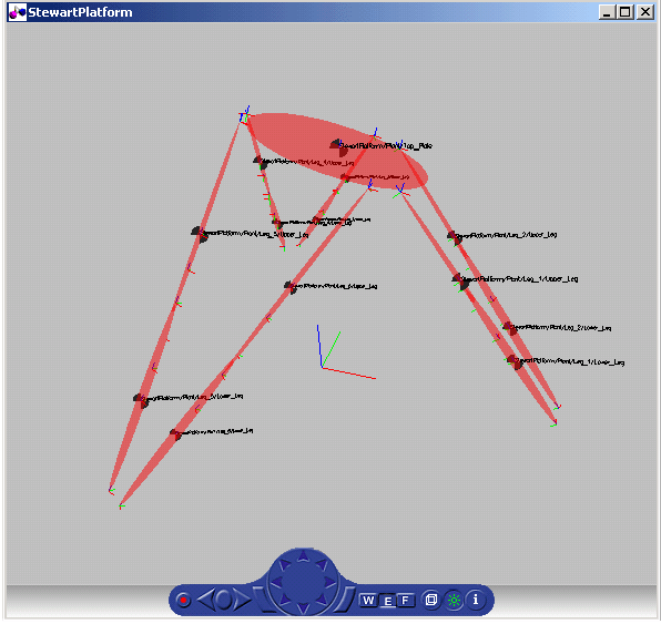
A more realistic way of visualizing the model can be done using the Virtual Reality Toolbox. The Virtual Reality Toolbox uses Virtual Reality Modeling Language (VRML), to create and populate virtual worlds with user-defined bodies. The simplest way to use the Virtual Reality Toolbox with SimMechanics is by selecting Virtual Reality Toolbox instead of MATLAB graphics under the Visualization tab of the Mechanical Environment Settings. This will provide the same options for body shapes that are available for MATLAB graphics. With Virtual Reality Toolbox selected, your default VRML viewer will open, showing a representation for the initial position of the model.
It is also possible to create or import a VRML scene of the Stewart Platform and hook it up to our Simulink and SimMechanics model using the Virtual Reality Toolbox blocks.
Future Directions
This article investigated the Stewart Platform, and how to create a model of the controller and mechanical components using SimMechanics. SimMechanics made it easy to build a hierarchical model of the mechanical plant and to modify the settings of the model. The model was trimmed and linearized using command-line functionality, demonstrating that it is easy to link the model with MATLAB advanced control design products. Most importantly, this example demonstrated how plant modeling, controller synthesis, and closed-loop simulation can all be performed within one environment.
There are other components of the Stewart Platform not explored in this example, such as linear motors, limit switches, and safety critical logic. These tasks could easily be performed using Simulink, Stateflow, SimMechanics, and SimPowerSystems.
Files required to run this example can be downloaded at MATLAB Central.
Published 2002
