多変量時系列の予想

ライブスクリプトを開く

この例では、被捕食者の群れのシナリオにおける捕食者個体群と被捕食者個体群から測定したデータについて、多変量時系列予想を実施する方法を説明します。捕食者個体群と被捕食者個体群の変化のダイナミクスを、線形および非線形の時系列モデルを使ってモデル化します。これらのモデルの予想のパフォーマンスを比較します。

データの説明

データは捕食者 1、被捕食者 1 の個体群 (千単位) で構成される二変量時系列で、20 年間にわたり毎年 10 回ずつ収集されたものです。データの詳細については、3 つの個体群生態系: 時系列の MATLAB と C MEX ファイルモデリングを参照してください。

時系列データを読み込みます。

load PredPreyCrowdingData
z = iddata(y,[],0.1,'TimeUnit','years','Tstart',0);

z は iddata オブジェクトであり、それぞれが捕食者個体群と被捕食者個体群を参照する 2 つの出力信号 y1 と y2 を含みます。z の OutputData プロパティには個体群データが 201 行 2 列の行列として含まれ、z.OutputData(:,1) は捕食者個体群、z.OutputData(:,2) は被捕食者個体群となります。

データをプロットします。

plot(z)
title('Predator-Prey Population Data')
ylabel('Population (thousands)')

Figure contains 2 axes objects. Axes object 1 with title y1 contains an object of type line. This object represents z. Axes object 2 with title y2 contains an object of type line. This object represents z.

データには、過密によって捕食者の個体数が減少することが示されています。

その最初の半分を推定用データとして使用して、系列モデルを同定します。

ze = z(1:120);

残りのデータはモデル次数の検索と予想結果の検証に使用します。

zv = z(121:end);

線形モデルの推定

時系列を線形の自己回帰過程としてモデル化します。線形モデルを多項式形式または状態空間形式で作成するには、ar (スカラー時系列のみ)、arx、armax、n4sid および ssest などのコマンドを使用します。線形モデルはデータのオフセットを捉えることができないので (非ゼロの条件付き平均)、まずデータからトレンドを除去します。

[zed, Tze] = detrend(ze, 0);
[zvd, Tzv] = detrend(zv, 0);

同定にはモデル次数の指定が必要です。多項式モデルの場合は、arxstruc コマンドを使用して、適切な次数を見つけることができます。arxstruc は単出力モデルでのみ機能するため、モデル次数の検索は出力ごとに別々に実行します。

na_list = (1:10)';
V1 = arxstruc(zed(:,1,:),zvd(:,1,:),na_list);
na1 = selstruc(V1,0);
V2 = arxstruc(zed(:,2,:),zvd(:,2,:),na_list);
na2 = selstruc(V2,0);

arxstruc コマンドは、それぞれ次数が 7 と 8 の自己回帰モデルを示しています。

これらのモデル次数を使用して、クロス項が任意に選択された多分散 ARMA モデルを推定します。

na = [na1 na1-1; na2-1 na2];
nc = [na1; na2];
sysARMA = armax(zed,[na nc])

sysARMA =
Discrete-time ARMA model:                                                                                    
  Model for output "y1": A(z)y_1(t) = - A_i(z)y_i(t) + C(z)e_1(t)                                            
    A(z) = 1 - 0.885 z^-1 - 0.1493 z^-2 + 0.8089 z^-3 - 0.2661 z^-4 - 0.9487 z^-5 + 0.8719 z^-6 - 0.2896 z^-7
                                                                                                             
    A_2(z) = 0.3433 z^-1 - 0.2802 z^-2 - 0.04949 z^-3 + 0.1018 z^-4 - 0.02683 z^-5 - 0.2416 z^-6             
                                                                                                             
    C(z) = 1 - 0.4534 z^-1 - 0.4127 z^-2 + 0.7874 z^-3 + 0.298 z^-4 - 0.8684 z^-5 + 0.6106 z^-6 + 0.3616 z^-7
                                                                                                             
  Model for output "y2": A(z)y_2(t) = - A_i(z)y_i(t) + C(z)e_2(t)                                                            
    A(z) = 1 - 0.5826 z^-1 - 0.4688 z^-2 - 0.5949 z^-3 - 0.0547 z^-4 + 0.5062 z^-5 + 0.4024 z^-6 - 0.01544 z^-7 - 0.1766 z^-8
                                                                                                                             
    A_1(z) = 0.2386 z^-1 + 0.1564 z^-2 - 0.2249 z^-3 - 0.2638 z^-4 - 0.1019 z^-5 - 0.07821 z^-6 + 0.2982 z^-7                
                                                                                                                             
    C(z) = 1 - 0.1717 z^-1 - 0.09877 z^-2 - 0.5289 z^-3 - 0.24 z^-4 + 0.06555 z^-5 + 0.2217 z^-6 - 0.05765 z^-7 - 0.1824 z^-8
                                                                                                                             
Sample time: 0.1 years
  
Parameterization:
   Polynomial orders:   na=[7 6;7 8]   nc=[7;8]
   Number of free coefficients: 43
   Use "polydata", "getpvec", "getcov" for parameters and their uncertainties.

Status:                                                  
Estimated using ARMAX on time domain data "zed".         
Fit to estimation data: [89.85;90.97]% (prediction focus)
FPE: 3.814e-05, MSE: 0.007533

10 ステップ先 (1 年後) の予測出力を計算して、推定データの時間範囲にわたるモデルの検証を行います。推定のためにデータのトレンド除去を行ったので、意味のある予測を得るためにそれらのオフセットを指定する必要があります。

predOpt = predictOptions('OutputOffset',Tze.OutputOffset');
yhat1 = predict(sysARMA,ze,10, predOpt);

predict コマンドは測定データの時間範囲にわたる応答を予測し、推定されたモデルの質を検証するためのツールになります。時間 t での応答は、t = 0、...、t-10 の時間での測定値を使って計算されます。

予測された応答と測定データをプロットします。

plot(ze,yhat1)
title('10-step predicted response compared to measured data')

$Figure contains 2 axes objects. Axes object 1 with title y1 contains 2 objects of type line. These objects represent ze, ze\_Predicted. Axes object 2 with title y2 contains 2 objects of type line. These objects represent ze, ze\_Predicted.$

予測された応答の生成と、それを測定データと併せたプロットは、compare コマンドを使用して自動化できます。

compareOpt = compareOptions('OutputOffset',Tze.OutputOffset');
compare(ze,sysARMA,10,compareOpt)

Figure contains 2 axes objects. Axes object 1 with ylabel y1 contains 2 objects of type line. These objects represent Validation data (y1), sysARMA: 75.49%. Axes object 2 with ylabel y2 contains 2 objects of type line. These objects represent Validation data (y2), sysARMA: 76.21%.

compare を使って生成したプロットには、パーセント形式で適合度を示す正規化された平方根平均二乗 (NRMSE) の測定値も示されます。

データを検証した後、推定データの 100 ステップ (10 年) 先におけるモデル sysARMA の出力を予想し、出力の標準偏差を計算します。

forecastOpt = forecastOptions('OutputOffset',Tze.OutputOffset');
[yf1,x01,sysf1,ysd1] = forecast(sysARMA, ze, 100, forecastOpt);

yf1 は予想された応答を iddata オブジェクトとして返したものです。yf1.OutputData には予想された値が含まれます。

sysf1 は sysARMA と類似したシステムですが、状態空間形式です。sim コマンドを使用して初期条件 x01 で sysf1 をシミュレートすることで、予想される応答 yf1 を再度生成します。

ysd1 は標準偏差の行列です。これは、データの加法性外乱の効果に起因する予想の不確かさ (sysARMA.NoiseVariance で測定)、パラメーターの不確かさ (getcov(sysARMA) で報告)、および過去のデータを予想に必要な初期条件にマッピングするプロセスに関連する不確かさ (data2state を参照) を測定します。

モデル sysARMA の測定出力、予測出力、予想出力をプロットします。

t = yf1.SamplingInstants;
te = ze.SamplingInstants;
t0 = z.SamplingInstants;
subplot(1,2,1);
plot(t0,z.y(:,1),...
   te,yhat1.y(:,1),...
   t,yf1.y(:,1),'m',...
   t,yf1.y(:,1)+ysd1(:,1),'k--', ...
   t,yf1.y(:,1)-ysd1(:,1), 'k--')
xlabel('Time (year)');
ylabel('Predator population, in thousands');
subplot(1,2,2);
plot(t0,z.y(:,2),...
   te,yhat1.y(:,2),...
   t,yf1.y(:,2),'m',...
   t,yf1.y(:,2)+ysd1(:,2),'k--', ...
   t,yf1.y(:,2)-ysd1(:,2),'k--')
% Make the figure larger.
fig = gcf;
p = fig.Position;
fig.Position = [p(1),p(2)-p(4)*0.2,p(3)*1.4,p(4)*1.2];
xlabel('Time (year)');
ylabel('Prey population, in thousands');
legend({'Measured','Predicted','Forecasted','Forecast Uncertainty (1 sd)'},...
   'Location','best')

Figure contains 2 axes objects. Axes object 1 with xlabel Time (year), ylabel Predator population, in thousands contains 5 objects of type line. Axes object 2 with xlabel Time (year), ylabel Prey population, in thousands contains 5 objects of type line. These objects represent Measured, Predicted, Forecasted, Forecast Uncertainty (1 sd).

プロットでは、線形 ARMA モデルを (オフセットの処理とともに) 使用した予想がある程度機能し、12 ～ 20 年の期間にわたる実際の個体数と比較した場合、その結果は不確かさが大きいことが示されています。これは、個体群変化のダイナミクスが非線形である可能性を示しています。

非線形ブラックボックスモデルの推定

この節では、モデルに非線形要素を追加することにより、前節のブラックボックス同定法を拡張します。これは、非線形 ARX モデリングフレームワークを使用して実行されます。非線形 ARX モデルは、次の 2 ステップのプロセスを使用して予測出力を計算するという点で、線形モデル (上記の sysARMA など) と概念的に類似しています。

測定信号を有限次元リグレッサー空間にマッピングします。
線形または非線形にできる静的関数を使用して、リグレッサーを予測出力にマッピングします。

非線形性は、リグレッサーセット (ステップ 1) および/または静的マッピング関数 (ステップ 2) という 2 か所のいずれかで追加できます。この節では、これらのオプションの両方について考えます。最初に、リグレッサーが線形型である非線形 ARX モデルを作成します。ここで、すべての非線形性はリグレッサー定義のみに制限され、リグレッサーを予測出力に変換する静的マッピング関数は線形 (厳密にいえばアフィン) です。次に、ガウス過程関数を静的マッピング関数として使用し、リグレッサーを線形に維持するモデルを作成します。

多項式 AR モデル

2 つの出力をもち入力なしの、非線形 ARX モデルを作成します。

L = linearRegressor(ze.OutputName,{1,1});
sysNLARX = idnlarx(ze.OutputName, ze.InputName, L, []);
sysNLARX.Ts = 0.1;
sysNLARX.TimeUnit = 'years';

sysNLARX は、非線形関数を使用しない 1 次の非線形 ARX モデルです。このモデルはその 1 次リグレッサーの加重合計を使ってモデル応答を予測します。

getreg(sysNLARX)

ans = 2x1 cell
    {'y1(t-1)'}
    {'y2(t-1)'}

非線形関数を導入するには、多項式のリグレッサーをモデルに追加します。

次数 2 のリグレッサーを作成し、クロス項 (上記の標準リグレッサーの積) を含めます。これらのリグレッサーをモデルに追加します。

P = polynomialRegressor(ze.OutputName,{1,1},2,false,true);
sysNLARX.Regressors(end+1) = P;
getreg(sysNLARX)

ans = 5x1 cell
    {'y1(t-1)'        }
    {'y2(t-1)'        }
    {'y1(t-1)^2'      }
    {'y2(t-1)^2'      }
    {'y1(t-1)*y2(t-1)'}

推定データ ze を使用してモデルの係数 (リグレッサーの重みとオフセット) を推定します。

sysNLARX = nlarx(ze,sysNLARX)

sysNLARX =

Nonlinear multivariate time series model with 2 outputs
  Outputs: y1, y2

Regressors:
  1. Linear regressors in variables y1, y2
  2. Order 2 regressors in variables y1, y2

Output functions:
  Output 1:  Linear with offset
  Output 2:  Linear with offset

Sample time: 0.1 years

Status:                                                       
Termination condition: Near (local) minimum, (norm(g) < tol)..
Number of iterations: 0, Number of function evaluations: 1    
                                                              
Estimated using NLARX on time domain data "ze".               
Fit to estimation data: [88.34;88.91]% (prediction focus)     
FPE: 3.265e-05, MSE: 0.01048                                  
More information in model's "Report" property.

10 ステップ先の予測出力を計算してモデルを検証します。

yhat2 = predict(sysNLARX,ze,10);

推定データの 100 ステップ先におけるモデルの出力を予想します。

yf2 = forecast(sysNLARX,ze,100);

非線形 ARX モデルでは、予想される応答の標準偏差が計算されません。このデータが提供されないのは、これらのモデルの推定時にパラメーター共分散の情報が計算されないためです。

測定出力、予測出力、予想出力をそれぞれプロットします。

t = yf2.SamplingInstants;
subplot(1,2,1);
plot(t0,z.y(:,1),...
   te,yhat2.y(:,1),...
   t,yf2.y(:,1),'m')
xlabel('Time (year)');
ylabel('Predator population (thousands)');
title('Prediction Results for ARX Model with Polynomial Regressors')
subplot(1,2,2);
plot(t0,z.y(:,2),...
   te,yhat2.y(:,2),...
   t,yf2.y(:,2),'m')
legend('Measured','Predicted','Forecasted')
xlabel('Time (year)');
ylabel('Prey population (thousands)');

Figure contains 2 axes objects. Axes object 1 with title Prediction Results for ARX Model with Polynomial Regressors, xlabel Time (year), ylabel Predator population (thousands) contains 3 objects of type line. Axes object 2 with xlabel Time (year), ylabel Prey population (thousands) contains 3 objects of type line. These objects represent Measured, Predicted, Forecasted.

プロットには、非線形 ARX モデルを使用した予想によって、線形モデルを使用した場合よりも良好な予想結果が得られることが示されています。非線形のブラックボックスモデリングでは、データを扱う方程式に関する事前情報が不要でした。

リグレッサーの数を減らすために、Statistics and Machine Learning Toolbox™ の主成分分析 (pca を参照) または特徴選択 (sequentialfs を参照) を使用して、最適な (変換された) 変数のサブセットを選択できる点に注意してください。

ガウス過程モデルの推定

モデル sysNLARX は線形マッピング関数を使用します。非線形性はリグレッサーのみに含まれます。より柔軟性のある方法には、ガウス過程関数 (GP) などの自明でないマッピング関数の選択が含まれます。線形リグレッサーのみを使用し、リグレッサーを出力にマッピングするガウス過程関数を追加する非線形 ARX モデルを作成します。

% Copy sysNLARX so we don't have to create the model structure again
sysGP = sysNLARX;
% Remove polynomial regressor set
sysGP.Regressors(2) = [];
% Replace the linear mapping function by a Gaussian Process (GP) function.
% The GP uses a squared exponential kernel by default.
GP = idGaussianProcess;
sysGP.OutputFcn = GP;
disp(sysGP)

  2x0 idnlarx array with properties:

        Regressors: [1x1 linearRegressor]
         OutputFcn: [2x1 idGaussianProcess]
    RegressorUsage: [2x4 table]
     Normalization: [1x1 struct]
      TimeVariable: 't'
     NoiseVariance: [2x2 double]
         InputName: {0x1 cell}
         InputUnit: {0x1 cell}
        InputGroup: [1x1 struct]
        OutputName: {2x1 cell}
        OutputUnit: {2x1 cell}
       OutputGroup: [1x1 struct]
             Notes: [0x1 string]
          UserData: []
              Name: ''
                Ts: 0.1000
          TimeUnit: 'years'
            Report: [1x1 idresults.nlarxhw]

これでテンプレートモデル sysGP は、線形リグレッサーおよび GP マッピング関数に基づきました。このパラメーターは、二乗指数カーネルの 2 つの係数です。nlarx を使用して、これらのパラメーターを推定します。

sysGP = nlarx(ze, sysGP)

sysGP =

Nonlinear multivariate time series model with 2 outputs
  Outputs: y1, y2

Regressors:
  Linear regressors in variables y1, y2

Output functions:
  Output 1:  Gaussian process function using a SquaredExponential kernel
  Output 2:  Gaussian process function using a SquaredExponential kernel

Sample time: 0.1 years

Status:                                                  
Estimated using NLARX on time domain data "ze".          
Fit to estimation data: [88.07;88.84]% (prediction focus)
FPE: 3.369e-05, MSE: 0.01083                             
More information in model's "Report" property.

getpvec(sysGP)

前と同様に、予測された応答および予想される応答を計算して、結果をプロットします。

10 ステップ先の予測出力を計算してモデルを検証します。

yhat3 = predict(sysGP,ze,10);

推定データの 100 ステップ先におけるモデルの出力を予想します。

yf3 = forecast(sysGP,ze,100);

測定出力、予測出力、予想出力をそれぞれプロットします。

t = yf3.SamplingInstants;
subplot(1,2,1);
plot(t0,z.y(:,1),...
   te,yhat3.y(:,1),...
   t,yf3.y(:,1),'m')
xlabel('Time (year)');
ylabel('Predator population (thousands)');
title('Prediction Results for Gaussian Process Model')
subplot(1,2,2);
plot(t0,z.y(:,2),...
   te,yhat3.y(:,2),...
   t,yf3.y(:,2),'m')
legend('Measured','Predicted','Forecasted')
xlabel('Time (year)');
ylabel('Prey population (thousands)');

Figure contains 2 axes objects. Axes object 1 with title Prediction Results for Gaussian Process Model, xlabel Time (year), ylabel Predator population (thousands) contains 3 objects of type line. Axes object 2 with xlabel Time (year), ylabel Prey population (thousands) contains 3 objects of type line. These objects represent Measured, Predicted, Forecasted.

結果は、線形モデル全体で精度が向上したことを示しています。GP に基づくモデルを使用する利点は、ウェーブレットネットワーク (idWaveletNetwork) またはシグモイドネットワーク (idSigmoidNetwork) などの他の形式と異なり、パラメーターをほとんど使用しないことです。これにより、パラメーター推定において、低い不確かさで学習が容易になります。

非線形グレーボックスモデルの推定

システムダイナミクスについての事前情報がある場合、非線形グレーボックスモデルを使用して推定データを当てはめることができます。ダイナミクスの性質に関する情報は、一般的に、モデルの品質と予想の正確性を改善するのに役立つことがあります。捕食者と被捕食者のダイナミクスの場合、捕食者 (y1) および被捕食者 (y2) の個体群における変化を次のように表すことができます。

${y_{}^{˙}}_{1} (t) = p_{1} * y_{1} (t) + p_{2} * y_{2} (t) * y_{1} (t)$

${y_{}^{˙}}_{2} (t) = p_{3} * y_{2} (t) - p_{4} * y_{1} (t) * y_{2} (t) - p_{5} * y_{2} (t)^{2}$

方程式の詳細については、3 つの個体群生態系: 時系列の MATLAB と C MEX ファイルモデリングを参照してください。

これらの方程式に基づいて非線形グレーボックスモデルを作成します。

捕食系のモデル構造を記述するファイルを指定します。このファイルは状態微分およびモデル出力を、時間、状態、入力およびモデルパラメーターの関数として指定します。ダイナミクスの非線形状態空間記述を導出するため、状態として 2 つの出力 (捕食者個体群と被捕食者個体群) が選択されます。

FileName = 'predprey2_m';

モデルの次数 (出力数、入力数および状態数) を指定します。

Order = [2 0 2];

$p_{1}$ 、 $p_{2}$ 、 $p_{3}$ 、 $p_{4}$ 、 $p_{5}$ の各パラメーターの初期値を指定し、すべてのパラメーターが推定されるように指示します。ブラックボックスモデル sysARMA および sysNLARX の推定時には、パラメーターの初期推定値は指定の必要がなかった点に注意してください。

Parameters = struct('Name',{'Survival factor, predators' 'Death factor, predators' ...
   'Survival factor, preys' 'Death factor, preys' ...
   'Crowding factor, preys'}, ...
   'Unit',{'1/year' '1/year' '1/year' '1/year' '1/year'}, ...
   'Value',{-1.1 0.9 1.1 0.9 0.2}, ...
   'Minimum',{-Inf -Inf -Inf -Inf -Inf}, ...
   'Maximum',{Inf Inf Inf Inf Inf}, ...
   'Fixed',{false false false false false});

同様に、モデルの初期状態を指定して、両方の初期状態が推定されるように指示します。

InitialStates = struct('Name',{'Predator population' 'Prey population'}, ...
   'Unit',{'Size (thousands)' 'Size (thousands)'}, ...
   'Value',{1.8 1.8}, ...
   'Minimum', {0 0}, ...
   'Maximum',{Inf Inf}, ...
   'Fixed',{false false});

モデルを連続時間システムとして指定します。

Ts = 0;

指定された構造、パラメーターおよび状態をもつ非線形グレーボックスモデルを作成します。

sysGrey = idnlgrey(FileName,Order,Parameters,InitialStates,Ts,'TimeUnit','years');

モデルのパラメーターを推定します。

sysGrey = nlgreyest(ze,sysGrey);
present(sysGrey)

                                                                                                                                                                                                                                                                                                                      
sysGreyGrey =                                                                                                                                                                                                                                                                                                         
                                                                                                                                                                                                                                                                                                                      
Continuous-time nonlinear grey-box model defined by 'predprey2_m' (MATLAB file):                                                                                                                                                                                                                                      
                                                                                                                                                                                                                                                                                                                      
   dx/dt = F(t, x(t), p1, ..., p5)                                                                                                                                                                                                                                                                                    
    y(t) = H(t, x(t), p1, ..., p5) + e(t)                                                                                                                                                                                                                                                                             
                                                                                                                                                                                                                                                                                                                      
 with 0 input(s), 2 state(s), 2 output(s), and 5 free parameter(s) (out of 5).                                                                                                                                                                                                                                        
                                                                                                                                                                                                                                                                                                                      
 States:                                        Initial value                                                                                                                                                                                                                                                         
    x(1)  Predator population(t) [Size (thou..]   xinit@exp1   2.01325   (estimated) in [0, Inf]                                                                                                                                                                                                                      
    x(2)  Prey population(t) [Size (thou..]       xinit@exp1   1.99687   (estimated) in [0, Inf]                                                                                                                                                                                                                      
 Outputs:                                                                                                                                                                                                                                                                                                             
    y(1)  y1(t)                                                                                                                                                                                                                                                                                                       
    y(2)  y2(t)                                                                                                                                                                                                                                                                                                       
 Parameters:                                    Value  Standard Deviation                                                                                                                                                                                                                                             
    p1   Survival factor, predators [1/year]     -0.995895      0.0125269   (estimated) in [-Inf, Inf]                                                                                                                                                                                                                
    p2   Death factor, predators [1/year]          1.00441      0.0129368   (estimated) in [-Inf, Inf]                                                                                                                                                                                                                
    p3   Survival factor, preys [1/year]           1.01234      0.0135413   (estimated) in [-Inf, Inf]                                                                                                                                                                                                                
    p4   Death factor, preys [1/year]              1.01909      0.0121026   (estimated) in [-Inf, Inf]                                                                                                                                                                                                                
    p5   Crowding factor, preys [1/year]          0.103244      0.0039285   (estimated) in [-Inf, Inf]                                                                                                                                                                                                                
                                                                                                                                                                                                                                                                                                                      
Status:                                                                                                                                                                                                                                                                                                               
Termination condition: Change in cost was less than the specified tolerance..                                                                                                                                                                                                                                         
Number of iterations: 6, Number of function evaluations: 7                                                                                                                                                                                                                                                            
                                                                                                                                                                                                                                                                                                                      
Estimated using Solver: ode45; Search: lsqnonlin on time domain data "ze".                                                                                                                                                                                                                                            
Fit to estimation data: [91.21;92.07]%                                                                                                                                                                                                                                                                                
FPE: 8.613e-06, MSE: 0.005713                                                                                                                                                                                                                                                                                         
More information in model's "Report" property.                                                                                                                                                                                                                                                                        
                                                                                                                                                                                                                                                                                                                      
Model Properties

10 ステップ先の予測出力を計算してモデルを検証します。

yhat4 = predict(sysGrey,ze,10);

推定データの 100 ステップ先におけるモデルの出力を予想して、出力の標準偏差を計算します。

[yf4,x04,sysf4,ysd4] = forecast(sysGrey,ze,100);

測定出力、予測出力、予想出力をそれぞれプロットします。

t = yf4.SamplingInstants;
subplot(1,2,1);
plot(t0,z.y(:,1),...
   te,yhat4.y(:,1),...
   t,yf4.y(:,1),'m',...
   t,yf4.y(:,1)+ysd4(:,1),'k--', ...
   t,yf4.y(:,1)-ysd4(:,1),'k--')
xlabel('Time (year)');
ylabel('Predator population (thousands)');
title('Prediction Results for Grey-Box Model')
subplot(1,2,2);
plot(t0,z.y(:,2),...
   te,yhat4.y(:,2),...
   t,yf4.y(:,2),'m',...
   t,yf4.y(:,2)+ysd4(:,2),'k--', ...
   t,yf4.y(:,2)-ysd4(:,2),'k--')

legend('Measured','Predicted','Forecasted','Forecast uncertainty (1 sd)')
xlabel('Time (years)');
ylabel('Prey population (thousands)');

Figure contains 2 axes objects. Axes object 1 with title Prediction Results for Grey-Box Model, xlabel Time (year), ylabel Predator population (thousands) contains 5 objects of type line. Axes object 2 with xlabel Time (years), ylabel Prey population (thousands) contains 5 objects of type line. These objects represent Measured, Predicted, Forecasted, Forecast uncertainty (1 sd).

プロットでは、非線形グレーボックスモデルを使用した予想から良好な結果が得られ、予想出力の不確かさが低いことが示されています。

予想のパフォーマンスの比較

同定されたモデル sysARMA、sysNLARX および sysGrey から取得した、予想される応答を比較します。最初の 2 つは離散時間モデルで、sysGrey は連続時間モデルです。

clf
plot(z,yf1,yf2,yf3,yf4)
legend({'Measured','ARMA','Polynomial AR','GP','Grey-Box'})
title('Forecasted Responses')
xlim([7 23])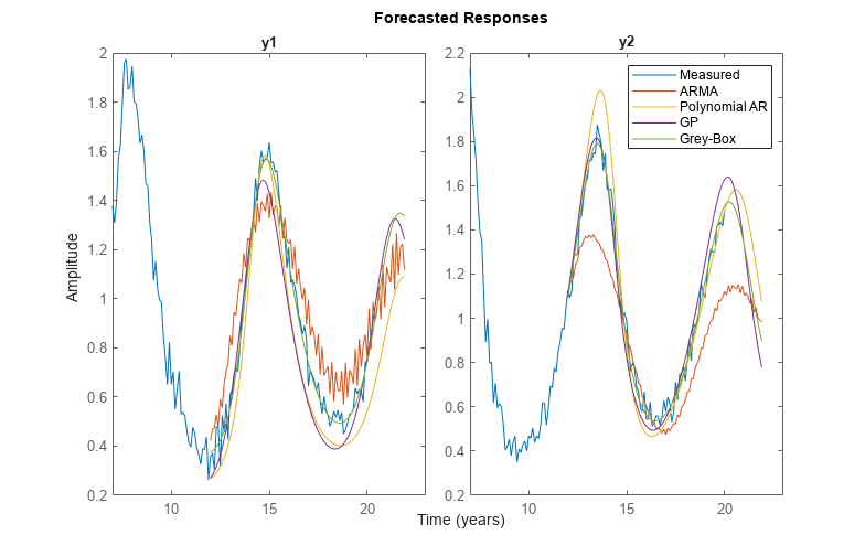

Figure contains 2 axes objects. Axes object 1 with title y1 contains 5 objects of type line. These objects represent Measured, ARMA, Polynomial AR, GP, Grey-Box. Axes object 2 with title y2 contains 5 objects of type line. These objects represent Measured, ARMA, Polynomial AR, GP, Grey-Box.

非線形 ARX モデルを使った予想では、線形モデルでの予想よりも良好な結果が得られます。非線形グレーボックスモデルにダイナミクスに関する情報を含めることで、モデルの信頼性はさらに改善され、予想の正確性は高まります。

グレーボックスモデリングで使われる方程式は、非線形 ARX モデルで使われる多項式リグレッサーと密接に関連している点に注意してください。基礎方程式内の導関数を 1 次差分で近似すると、以下に類似した方程式が得られます。

$y_{1} (t) = s_{1} * y_{1} (t - 1) + s_{2} * y_{1} (t - 1) * y_{2} (t - 1)$

$y_{2} (t) = s_{3} * y_{2} (t - 1) - s_{4} * y_{1} (t - 1) * y_{2} (t - 1) - s_{5} * y_{2} (t - 1)^{2}$

ここで、 $s_{1}, . . ., s_{5}$ は元のパラメーター $p_{1}, . . ., p_{5}$ および差分に使われるサンプル時間に関連するいくつかのパラメーターです。これらの方程式は、非線形 ARX モデルの作成に際して、最初の出力に必要なリグレッサーは y1(t-1) と *y1(t-1)*y2(t-1) の 2 つだけであり、2 番目の出力に必要なのは 3 つであることを示唆しています。このような事前情報がない場合でも、多項式リグレッサーを使用しリグレッサーが線形であるモデル構造が、実際上よく使用される選択肢であることに変わりはありません。

非線形グレーボックスモデルを使用して 200 年間にわたる値を予想します。

[yf5,~,~,ysd5] = forecast(sysGrey, ze, 2000);

1 sd の不確かさを示す、データの後半部分をプロットします。

t = yf5.SamplingInstants;
N = 700:2000;
subplot(1,2,1);
plot(t(N), yf5.y(N,1), 'm',...
   t(N), yf5.y(N,1)+ysd5(N,1), 'k--', ...
   t(N), yf5.y(N,1)-ysd5(N,1), 'k--')
xlabel('Time (year)');
ylabel('Predator population (thousands)');
title('Forecasted Population after 200 Years')
ax = gca;
ax.YLim = [0.8 1];
ax.XLim = [82 212];
subplot(1,2,2);
plot(t(N),yf5.y(N,2),'m',...
   t(N),yf5.y(N,2)+ysd5(N,2),'k--', ...
   t(N),yf5.y(N,2)-ysd5(N,2),'k--')
legend('Forecasted population','Forecast uncertainty (1 sd)')
xlabel('Time (years)');
ylabel('Prey population (thousands)');
ax = gca;
ax.YLim = [0.9 1.1];
ax.XLim = [82 212];

Figure contains 2 axes objects. Axes object 1 with title Forecasted Population after 200 Years, xlabel Time (year), ylabel Predator population (thousands) contains 3 objects of type line. Axes object 2 with xlabel Time (years), ylabel Prey population (thousands) contains 3 objects of type line. These objects represent Forecasted population, Forecast uncertainty (1 sd).

プロットには、捕食者数が約 890 で定常状態に達し、被捕食者数は 990 に達するという予想が示されています。

多変量時系列の予想

データの説明

線形モデルの推定

非線形ブラックボックス モデルの推定

多項式 AR モデル

ガウス過程モデルの推定

非線形グレー ボックス モデルの推定

予想のパフォーマンスの比較

関連するトピック

非線形ブラックボックスモデルの推定

非線形グレーボックスモデルの推定