各種のモデル同定法の比較

ライブスクリプトを開く

この例では、System Identification Toolbox™ で使用できる複数の同定法を紹介します。まず最初に、実験データをシミュレートし、複数の推定手法を使用して、このデータからモデルを推定します。この例では spa、ssest、tfest、arx、oe、armax、bj の各推定ルーチンが使用されています。

システムの説明

ノイズで破損された線形システムは、以下のように表されます。

y = G u + H e

ここで、y は出力、u は入力を示し、e は測定されていない (ホワイト) ノイズ源を意味します。G はシステムの伝達関数、H はノイズによる外乱の記述を示します。

G と H を推定する方法はたくさんあります。基本的に、この 2 つは、これらの関数をパラメーター化する各種の方法に対応します。

モデルの定義

System Identification Toolbox では、物理プロセスから取得した場合のデータをシミュレートするオプションが使用できます。一連の係数で IDPOLY モデルからのデータをシミュレートしてみましょう。

B = [0 1 0.5];
A = [1 -1.5 0.7];
m0 = idpoly(A,B,[1 -1 0.2],'Ts',0.25,'Variable','q^-1'); % The sample time is 0.25 s.

3 番目の引数 [1 -1 0.2] は、システムに影響を及ぼす外乱の特性を示します。以下のコマンドを実行すると、以下の離散時間 idpoly モデルが作成されます。

m0

m0 =
Discrete-time ARMAX model: A(q)y(t) = B(q)u(t) + C(q)e(t)
  A(q) = 1 - 1.5 q^-1 + 0.7 q^-2                         
                                                         
  B(q) = q^-1 + 0.5 q^-2                                 
                                                         
  C(q) = 1 - q^-1 + 0.2 q^-2                             
                                                         
Sample time: 0.25 seconds
  
Parameterization:
   Polynomial orders:   na=2   nb=2   nc=2   nk=1
   Number of free coefficients: 6
   Use "polydata", "getpvec", "getcov" for parameters and their uncertainties.

Status:                                                         
Created by direct construction or transformation. Not estimated.

ここで、q はシフト演算子を表し、A(q)y(t) は実際には、y(t) - 1.5 y(t-1) + 0.7 y(t-2) の短縮形です。モデル m0 の表示は、このモデルが ARMAX モデルであることを示しています。

このようなモデル構造は、ARMAX モデルと呼ばれ、AR (Autoregressive: 自己回帰) は、A- 多項式、MA (Moving average: 移動平均) はノイズ C- 多項式、および X は "eXtra " 入力 B(q)u(t) を表します。

一般的な伝達関数 G および H では、このモデルは以下のパラメーター化に対応します。

G(q) = B(q)/A(q) および H(q) = C(q)/A(q)、共通分母を含む

モデルのシミュレーション

入力信号 u を出力し、これらの入力に対するモデルの応答をシミュレートします。idinput コマンドを使用するとモデルへの入力信号を作成することができ、iddata コマンドを使用すると信号が適切な形式にパッケージ化されます。続いて、sim コマンドを使用して、以下のように出力をシミュレーションできます。

prevRng = rng(12,'v5normal');
u = idinput(350,'rbs');  %Generates a random binary signal of length 350
u = iddata([],u,0.25);   %Creates an IDDATA object. The sample time is 0.25 sec.
y = sim(m0,u,'noise')    %Simulates the model's response for this

y =

Time domain data set with 350 samples.
Sample time: 0.25 seconds              
Name: m0                               
                                       
Outputs      Unit (if specified)       
   y1

                         %input with added white Gaussian noise e
                         %according to the model description m0
rng(prevRng);

信号 u および y は、いずれも IDDATA オブジェクトです。次に、この入力/出力データを収集し、1 つの iddata オブジェクトを構成します。

z = [y,u];

このデータオブジェクト (この時点では、入力/出力データサンプルの両方を含む) に関する情報を取得するには、MATLAB® コマンドウィンドウにデータオブジェクトの名前を入力します。

z =

Time domain data set with 350 samples.
Sample time: 0.25 seconds              
Name: m0                               
                                       
Outputs      Unit (if specified)       
   y1                                  
                                       
Inputs       Unit (if specified)       
   u1

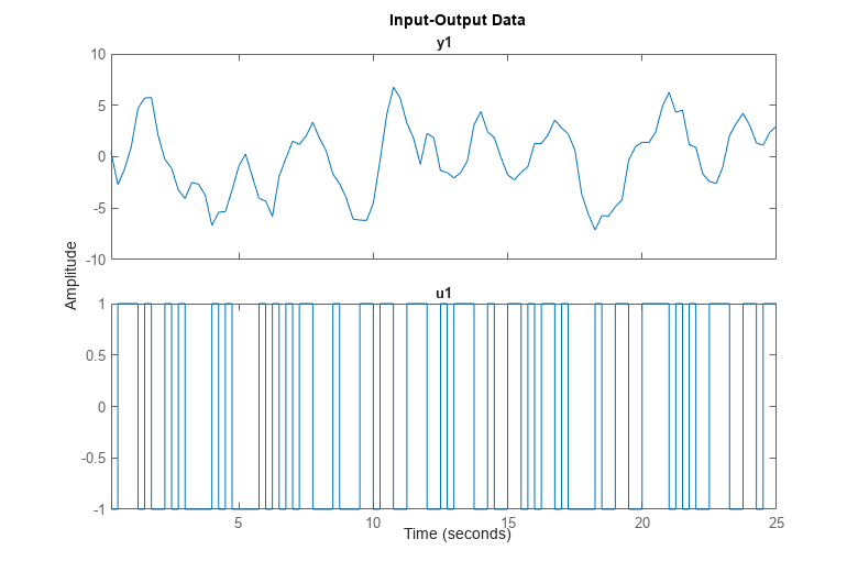
入力 u および出力 y の最初の 100 値をプロットするには、iddata オブジェクトで plot コマンドを使用します。

h = gcf; set(h,'DefaultLegendLocation','best')
h.Position = [100 100 780 520];
plot(z(1:100));

Figure contains 2 axes objects. Axes object 1 with title y1 contains an object of type line. This object represents m0. Axes object 2 with title u1 contains an object of type line. This object represents m0.

推定にはデータの一部だけを使用し (ze)、その他の部分は、後で推定モデルを検証するために残しておくことをお勧めします。

ze = z(1:200);
zv = z(201:350);

スペクトル解析の実行

シミュレートしたデータを取得できたので、モデルを推定して比較することができます。まず、スペクトル解析を実行してみましょう。ここでは、spa コマンドを使用します。このコマンドは、ノイズスペクトルと周波数関数のスペクトル解析推定を返します。

GS = spa(ze);

スペクトル解析の結果は、次の周波数の複素数関数となります。周波数応答。この値は、IDFRD (同定された周波数応答データ) オブジェクトにパッケージ化されます。

GS

GS =

IDFRD model.
Contains Frequency Response Data for 1 output(s) and 1 input(s), and the spectra for disturbances at the outputs.
Response data and disturbance spectra are available at 128 frequency points, ranging from 0.09817 rad/s to 12.57 rad/s.
 
Sample time: 0.25 seconds
Output channels: 'y1'
Input channels: 'u1'
Status:                                      
Estimated using SPA on time domain data "m0".

周波数応答をプロットするには通常、bode コマンドまたは bodeplot コマンドによるボード線図を使用します。

clf
h = bodeplot(GS); % bodeplot returns a plot handle, which bode does not
ax = axis; axis([0.1 10 ax(3:4)])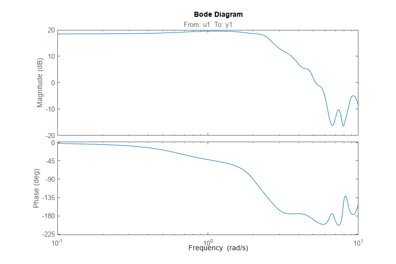

Figure contains 2 axes objects. Axes object 1 with title From: u1 To: y1, ylabel Magnitude (dB) contains an object of type line. This object represents GS. Axes object 2 with ylabel Phase (deg) contains an object of type line. This object represents GS.

ノイズで破損されたデータから作成されたため、推定値 GS は不確実です。また、スペクトル解析法では、このような不確かさを独自に評価できます。不確かさを表示するには (たとえば、標準偏差 3)、前の bodeplot コマンドで返されたプロットハンドル h で showConfidence コマンドを使用します。

showConfidence(h,3)

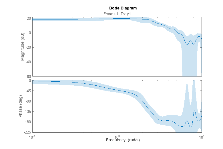
このプロットは、周波数応答のノミナル推定 (青線) は必ずしも正確ではないが、実応答が影付き (薄青) 領域内である確率は 99.7% (正規分布の標準偏差 3) であることを示します。

パラメトリック状態空間モデルの推定

続いて、(特定のモデル構造を指定しない) 既定の線形モデルを推定します。この場合、予測誤差法を使用して、状態空間モデルとして算出します。ここでは、関数 ssest を使用します。

m = ssest(ze) % The order of the model will be chosen automatically

m =
  Continuous-time identified state-space model:
      dx/dt = A x(t) + B u(t) + K e(t)
       y(t) = C x(t) + D u(t) + e(t)
 
  A = 
              x1         x2
   x1  -0.007167      1.743
   x2     -2.181     -1.337
 
  B = 
            u1
   x1  0.09388
   x2   0.2408
 
  C = 
          x1     x2
   y1  47.34  -14.4
 
  D = 
       u1
   y1   0
 
  K = 
             y1
   x1   0.04108
   x2  -0.03751
 
Parameterization:
   FREE form (all coefficients in A, B, C free).
   Feedthrough: none
   Disturbance component: estimate
   Number of free coefficients: 10
   Use "idssdata", "getpvec", "getcov" for parameters and their uncertainties.

Status:                                          
Estimated using SSEST on time domain data "m0".  
Fit to estimation data: 75.08% (prediction focus)
FPE: 0.9835, MSE: 0.9262

この時点で、状態空間モデルの行列には、あまり意味がありません。モデル m の周波数応答を、スペクトル解析推定 GS の周波数応答と比較できました。GS は離散時間モデルで、m は連続時間モデルです。ssest を使用して離散時間モデルを計算することもできます。

bodeplot(m,GS)
ax = axis; axis([0.1 10 ax(3:4)])

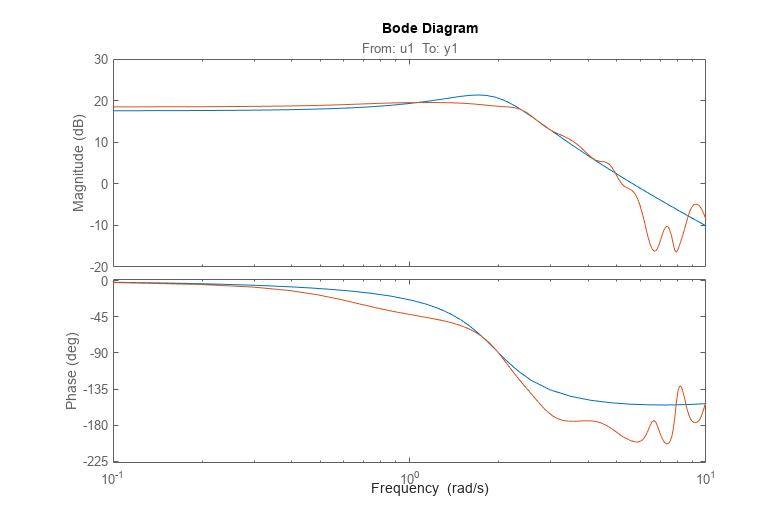
Figure contains 2 axes objects. Axes object 1 with title From: u1 To: y1, ylabel Magnitude (dB) contains 2 objects of type line. These objects represent m, GS. Axes object 2 with ylabel Phase (deg) contains 2 objects of type line. These objects represent m, GS.

2 つの周波数応答は、異なる方法で推定したにもかかわらず、非常に近いものとなります。

簡単な伝達関数の推定

線形モデル構造にはさまざまな種類がありますが、いずれも u と y の関係を記述する線形差分方程式または微分方程式に対応します。各構造はすべて、ノイズの影響をモデル化するさまざまな方法に対応します。これらのモデルの中で最も簡単なものは、伝達関数および ARX モデルです。伝達関数は次のような形式になります。

Y(s) = NUM(s)/DEN(s) U(s) + E(s)

ここで、NUM(s) と DEN(s) はそれぞれ分子多項式と分母多項式で、Y(s)、U(s)、E(s) はそれぞれ出力信号、入力信号、誤差信号 (y(t)、u(t)、e(t)) のラプラス変換です。NUM と DEN は、零点と極の数を表す次数によりパラメーター化できます。指定された極と零点の数から、tfest コマンドを使用して伝達関数を推定することができます。

mtf = tfest(ze, 2, 2) % transfer function with 2 zeros and 2 poles

mtf =
  From input "u1" to output "y1":
  -0.05428 s^2 - 0.02386 s + 29.6
  -------------------------------
       s^2 + 1.361 s + 4.102
 
Continuous-time identified transfer function.

Parameterization:
   Number of poles: 2   Number of zeros: 2
   Number of free coefficients: 5
   Use "tfdata", "getpvec", "getcov" for parameters and their uncertainties.

Status:                                        
Estimated using TFEST on time domain data "m0".
Fit to estimation data: 71.69%                 
FPE: 1.282, MSE: 1.195

ARX モデルは次のように表されます。A(q)y(t) = B(q)u(t) + e(t)、

または、完全に表記すると、

$y (t) + a_{1}^{} y (t - 1) + {\dots + a}_{na}^{} y (t - na) = b_{1}^{} u (t - nk) + \dots b_{nb}^{} u (t - nb - nk + 1) + e (t)$

このモデルの係数は線形です。係数 $a_{1}^{}$ 、 $a_{2}^{}$ 、...、 $b_{1}^{}$ 、 $b_{2}^{}$ 、... は最小二乗推定法を使用すると効率的に計算できます。規定の構造 (入力上で 2 つの極、1 つの零点および 1 つのラグ) をもつ ARX モデルの推定は、([na nb nk] = [2 2 1]) として取得されます。

mx = arx(ze,[2 2 1])

mx =
Discrete-time ARX model: A(z)y(t) = B(z)u(t) + e(t)
  A(z) = 1 - 1.32 z^-1 + 0.5393 z^-2               
                                                   
  B(z) = 0.9817 z^-1 + 0.4049 z^-2                 
                                                   
Sample time: 0.25 seconds
  
Parameterization:
   Polynomial orders:   na=2   nb=2   nk=1
   Number of free coefficients: 4
   Use "polydata", "getpvec", "getcov" for parameters and their uncertainties.

Status:                                          
Estimated using ARX on time domain data "m0".    
Fit to estimation data: 68.18% (prediction focus)
FPE: 1.603, MSE: 1.509

推定モデルの性能の比較

これらのモデル (mtf、mx) は既定の状態空間モデル m よりも良いでしょうか、悪いでしょうか。これを把握する 1 つの方法として、各モデル (ノイズなし) を検証データ zv の入力でシミュレートし、対応するシミュレートした出力をセット zv の測定出力と比較することが考えられます。

compare(zv,m,mtf,mx)

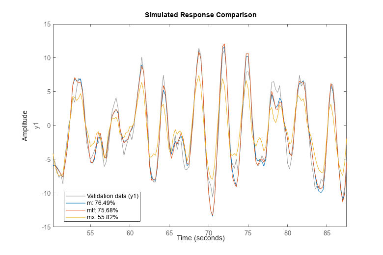
Figure contains an axes object. The axes object with ylabel y1 contains 4 objects of type line. These objects represent Validation data (y1), m: 76.49%, mtf: 75.68%, mx: 55.82%.

適合は、モデルに示される出力偏差のパーセントとなります。明らかに、m のほうがモデルとして優れていますが、mtf もこれに近い結果となります。離散時間伝達関数は tfest コマンドまたは oe コマンドを使用して推定できます。前者は IDTF モデルを作成し、後者は出力誤差構造 (y(t) = B(q)/F(q)u(t) + e(t)) の IDPOLY モデルを作成しますが、数学的には両者は同等です。

md1 = tfest(ze,2,2,'Ts',0.25)  % two poles and 2 zeros (counted as roots of polynomials in z^-1)

md1 =
  From input "u1" to output "y1":
   0.8383 z^-1 + 0.7199 z^-2
  ----------------------------
  1 - 1.497 z^-1 + 0.7099 z^-2
 
Sample time: 0.25 seconds
Discrete-time identified transfer function.

Parameterization:
   Number of poles: 2   Number of zeros: 2
   Number of free coefficients: 4
   Use "tfdata", "getpvec", "getcov" for parameters and their uncertainties.

Status:                                        
Estimated using TFEST on time domain data "m0".
Fit to estimation data: 71.46%                 
FPE: 1.264, MSE: 1.214

md2 = oe(ze,[2 2 1])

md2 =
Discrete-time OE model: y(t) = [B(z)/F(z)]u(t) + e(t)
  B(z) = 0.8383 z^-1 + 0.7199 z^-2                   
                                                     
  F(z) = 1 - 1.497 z^-1 + 0.7099 z^-2                
                                                     
Sample time: 0.25 seconds
  
Parameterization:
   Polynomial orders:   nb=2   nf=2   nk=1
   Number of free coefficients: 4
   Use "polydata", "getpvec", "getcov" for parameters and their uncertainties.

Status:                                     
Estimated using OE on time domain data "m0".
Fit to estimation data: 71.46%              
FPE: 1.264, MSE: 1.214

compare(zv, md1, md2)

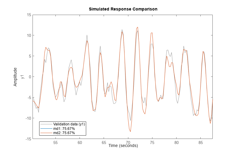
Figure contains an axes object. The axes object with ylabel y1 contains 3 objects of type line. These objects represent Validation data (y1), md1: 75.67%, md2: 75.67%.

モデル md1 および md2 は、データに対して同一の適合になります。

残差分析

モデルの特性についてさらに詳しく知るには、"残差" を算出します。すなわち、y = Gu + He において、モデルで示されない部分 e を計算します。理想的には、これらの値が入力と相関しておらず、お互いも相関しないことが望まれます。resid コマンドにより残差が算出され、その相関プロパティが表示されます。この関数は、時間領域と周波数領域の両方で残差を評価するときに使用できます。まず、時間領域で、出力誤差モデルの残差を取得しましょう。

resid(zv,md2) % plots the result of residual analysis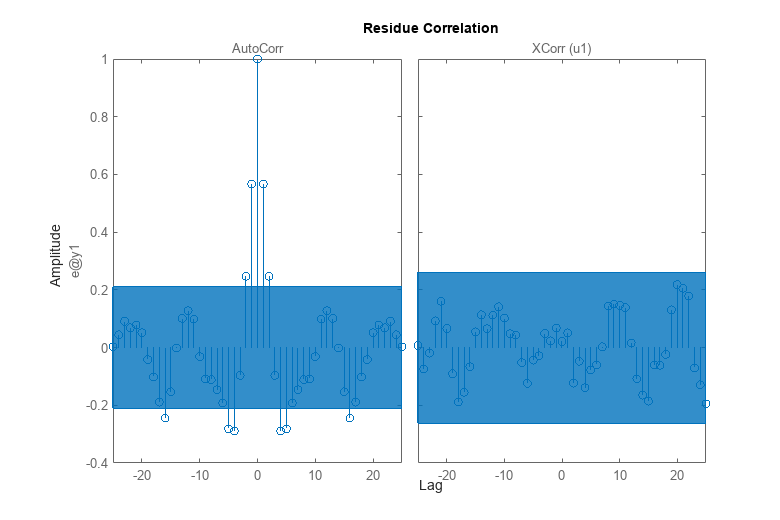

Figure contains 2 axes objects. Axes object 1 with title AutoCorr, ylabel e@y1 contains 2 objects of type line. One or more of the lines displays its values using only markers This object represents md2. Axes object 2 with title XCorr (u1) contains 2 objects of type line. One or more of the lines displays its values using only markers This object represents md2.

残差と入力の相互相関が信頼領域内にあり、有意な相関がないことが示されます。さらに、ダイナミクス G の推定を必要に応じて評価する必要があります。ただし、e の (自動) 相関は有意であり、e をホワイトノイズと見なすことはできません。これはつまり、ノイズモデル H が適切でないことを意味します。

ARMAX および Box-Jenkins モデルの推定

2 次 ARMAX モデルと 2 次 Box-Jenkins モデルを算出してみましょう。ARMAX モデルは、シミュレートしたモデル m0 と同様のノイズ特性をもち、Box-Jenkins モデルでは、より一般的なノイズ記述が可能です。

am2 = armax(ze,[2 2 2 1])  % 2nd order ARMAX model

am2 =
Discrete-time ARMAX model: A(z)y(t) = B(z)u(t) + C(z)e(t)
  A(z) = 1 - 1.516 z^-1 + 0.7145 z^-2                    
                                                         
  B(z) = 0.982 z^-1 + 0.5091 z^-2                        
                                                         
  C(z) = 1 - 0.9762 z^-1 + 0.218 z^-2                    
                                                         
Sample time: 0.25 seconds
  
Parameterization:
   Polynomial orders:   na=2   nb=2   nc=2   nk=1
   Number of free coefficients: 6
   Use "polydata", "getpvec", "getcov" for parameters and their uncertainties.

Status:                                          
Estimated using ARMAX on time domain data "m0".  
Fit to estimation data: 75.08% (prediction focus)
FPE: 0.9837, MSE: 0.9264

bj2 = bj(ze,[2 2 2 2 1])   % 2nd order BOX-JENKINS model

bj2 =
Discrete-time BJ model: y(t) = [B(z)/F(z)]u(t) + [C(z)/D(z)]e(t)
  B(z) = 0.9922 z^-1 + 0.4701 z^-2                              
                                                                
  C(z) = 1 - 0.6283 z^-1 - 0.1221 z^-2                          
                                                                
  D(z) = 1 - 1.221 z^-1 + 0.3798 z^-2                           
                                                                
  F(z) = 1 - 1.522 z^-1 + 0.7243 z^-2                           
                                                                
Sample time: 0.25 seconds
  
Parameterization:
   Polynomial orders:   nb=2   nc=2   nd=2   nf=2   nk=1
   Number of free coefficients: 8
   Use "polydata", "getpvec", "getcov" for parameters and their uncertainties.

Status:                                          
Estimated using BJ on time domain data "m0".     
Fit to estimation data: 75.47% (prediction focus)
FPE: 0.9722, MSE: 0.8974

推定モデルの比較 - シミュレーションと予測動作

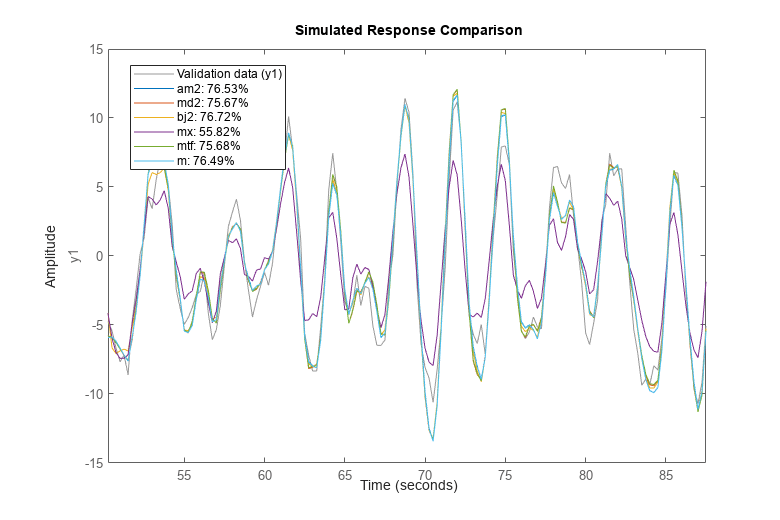
既に多数のモデルを推定したので、その一部を比較してみましょう。既にシミュレートした出力を比べることで、モデルを比較できます。

clf
compare(zv,am2,md2,bj2,mx,mtf,m)

Figure contains an axes object. The axes object with ylabel y1 contains 7 objects of type line. These objects represent Validation data (y1), am2: 76.53%, md2: 75.67%, bj2: 76.72%, mx: 55.82%, mtf: 75.68%, m: 76.49%.

また、推定された各種のモデルが、出力 (1 ステップ先の出力など) をどの程度正確に予測できるかも比較できます。

compare(zv,am2,md2,bj2,mx,mtf,m,1)

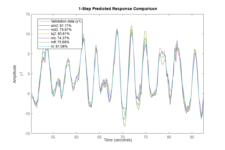
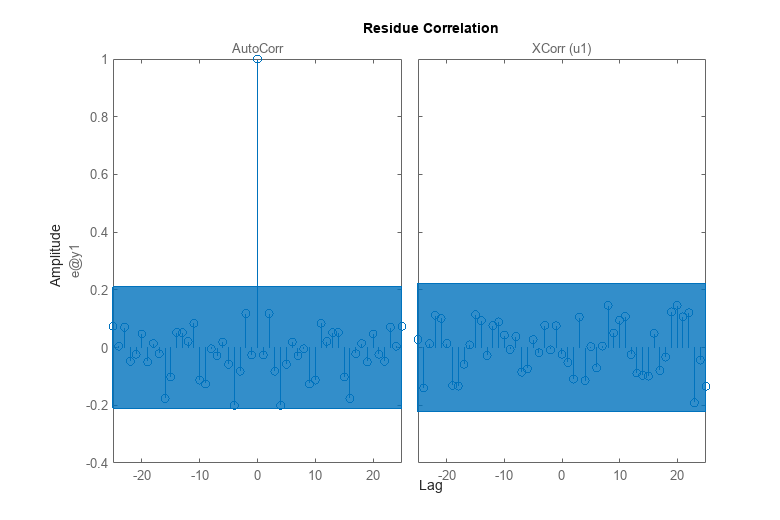
Figure contains an axes object. The axes object with ylabel y1 contains 7 objects of type line. These objects represent Validation data (y1), am2: 81.11%, md2: 75.67%, bj2: 80.81%, mx: 74.37%, mtf: 75.68%, m: 81.08%.

モデル bj2 の残差分析は、予測誤差には何の情報もないことを示しています。自己相関は見られず、入力とは無相関です。これは、Box-Jenkins モデル (C および D 多項式) の追加の動的要素でノイズダイナミクスを再現できたことを表しています。

resid(zv,bj2)

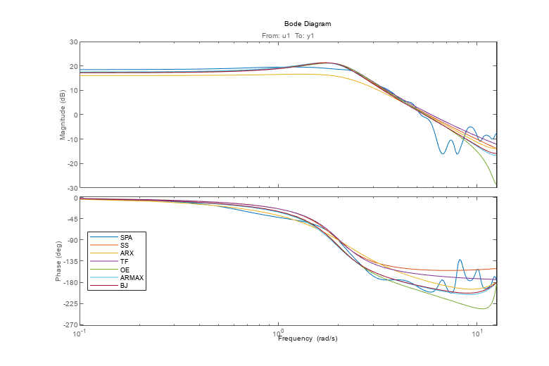
Figure contains 2 axes objects. Axes object 1 with title AutoCorr, ylabel e@y1 contains 2 objects of type line. One or more of the lines displays its values using only markers This object represents bj2. Axes object 2 with title XCorr (u1) contains 2 objects of type line. One or more of the lines displays its values using only markers This object represents bj2.

周波数関数の比較

作成したモデルで周波数関数を比較する場合にも、bodeplot コマンドを使用します。

clf
opt = bodeoptions; opt.PhaseMatching = 'on';
w = linspace(0.1,4*pi,100);
bodeplot(GS,m,mx,mtf,md2,am2,bj2,w,opt);
legend({'SPA','SS','ARX','TF','OE','ARMAX','BJ'},'Location','West');

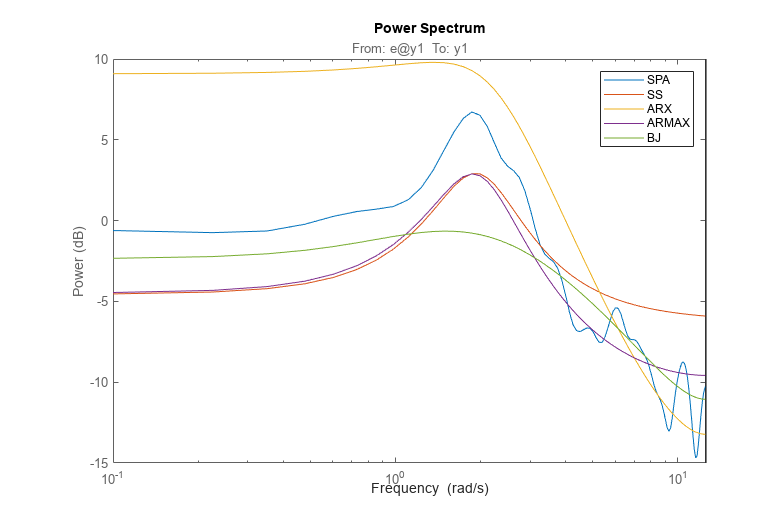
Figure contains 2 axes objects. Axes object 1 with title From: u1 To: y1, ylabel Magnitude (dB) contains 7 objects of type line. These objects represent SPA, SS, ARX, TF, OE, ARMAX, BJ. Axes object 2 with ylabel Phase (deg) contains 7 objects of type line. These objects represent SPA, SS, ARX, TF, OE, ARMAX, BJ.

また、推定モデルのノイズスペクトルも解析できます。たとえば、ARMAX および Box-Jenkins モデルのノイズスペクトルを、状態空間およびスペクトル解析モデルと比較します。ここでは、spectrum コマンドを使用します。

spectrum(GS,m,mx,am2,bj2,w)
legend('SPA','SS','ARX','ARMAX','BJ');

Figure contains an axes object. The axes object with title From: e@y1 To: y1, ylabel Power (dB) contains 5 objects of type line. These objects represent SPA, SS, ARX, ARMAX, BJ.

真のシステムと推定モデルの比較

推定モデルを、入出力データのシミュレートに使用した真のシステム m0 に対して検証します。ARMAX モデルの周波数関数を真のシステムと比較してみましょう。

bode(m0,am2,w)

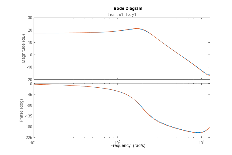
Figure contains 2 axes objects. Axes object 1 with title From: u1 To: y1, ylabel Magnitude (dB) contains 2 objects of type line. These objects represent m0, am2. Axes object 2 with ylabel Phase (deg) contains 2 objects of type line. These objects represent m0, am2.

応答はほぼ一致します。また、ノイズスペクトルを比較することもできます。

spectrum(m0,am2,w)

Figure contains an axes object. The axes object with title From: e@y1 To: y1, ylabel Power (dB) contains 2 objects of type line. These objects represent m0, am2.

極-零点プロットも評価してみましょう。

h = iopzplot(m0,am2);

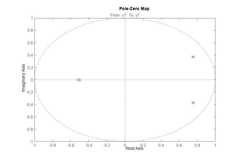
Figure contains an axes object. The axes object with title From: u1 To: y1 contains 4 objects of type line. One or more of the lines displays its values using only markers These objects represent m0, am2.

真のシステム (青) と ARMAX モデル (緑) の極と零点は、非常に近接していることがわかります。

さらに、零点と極の不確かさも評価できます。標準偏差 3 の値に対応する推定極および零点に関連する信頼領域をプロットするには、showConfidence を使用するか、プロットのコンテキスト (右クリック) メニューで [信頼領域] 特性をオンにします。

showConfidence(h,3)

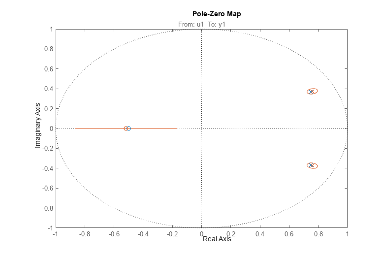
Figure contains an axes object. The axes object with title From: u1 To: y1 contains 8 objects of type line. One or more of the lines displays its values using only markers These objects represent m0, am2.

真のシステムの青い零点と極が、緑の不確実領域内に十分入っていることがわかります。