このページの内容は最新ではありません。最新版の英語を参照するには、ここをクリックします。
2 チャネル フィルター バンクによる再構成
この例では、完全再構成 2 チャネル フィルター バンクの設計法を示します。これは、直交ミラー フィルター (QMF) バンクとも呼ばれます。QMF バンクは電力相補フィルターを使用します。
デジタル信号処理において、まず低周波数サブバンドおよび高周波数サブバンドに信号を分割し、次にオリジナルの信号を再構成するためにこれらのサブバンドを組み合わせるという用途がいくつかあります。そのような用途の 1 つがサブバンド符号化 (SBC) です。
まずスケーリングされ時間シフトされたインパルスで構成される信号をフィルター処理して、完全再構成のプロセスをシミュレーションします。次に、システム全体の伝達関数の振幅スペクトルに加え、入力信号、出力信号およびエラー信号をプロットしますこの例で説明するフィルター バンクを通じて完全再構成の効果が示されます。
完全再構成
システムの出力が入力信号、または入力信号の遅延バージョンと等しい場合、そのシステムは完全再構成を実現していると言われます。以下は、理想フィルターを使用して信号をその低周波数成分と高周波数成分に分離し、信号を完全に復元する完全再構成プロセスのブロック線図です。完全な再構成プロセスには、4 つのフィルター、2 つのローパス フィルター ( と )、および 2 つのハイパス フィルター ( と ) が必要です。さらに、2 つのローパス フィルター間と 2 つのハイパス フィルター間には、ダウンサンプラーとアップサンプラーが必要です。解析フィルターには単位ゲインがあるので、合成フィルターはゲインを 2 とすることで先行するアップサンプラーを補正します。
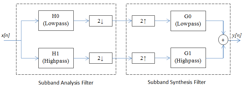
完全再構成 2 チャネル フィルター バンク
DSP System Toolbox™ には、FIR 完全再構成 2 チャネル フィルター バンクを実装するために必要な 4 つのフィルターを設計するために、firpr2chfb と呼ばれる特殊な関数が用意されています。関数 firpr2chfb は、2 チャネル完全再構成フィルター バンクの解析 ( と ) および合成 ( と ) セクション用に 4 つの FIR フィルターを設計します。設計は、完全再構成を実現するために必要な、直交フィルター バンク (電力対称フィルター バンクと呼ばれる) に対応します。
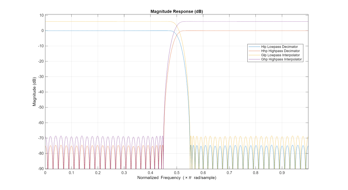
フィルター バンクを次数 99 のフィルター、およびローパス フィルター (0.45) とハイパス フィルター (0.55) の通過帯域エッジを使用して設計します。
N = 99;
[LPAnalysis, HPAnalysis, LPSynthsis, HPSynthesis] = firpr2chfb(N, 0.45);
次に、これらのフィルターの振幅応答をプロットします。
fvt = fvtool(LPAnalysis,1, HPAnalysis,1, LPSynthsis,1, HPSynthesis,1);
fvt.Color = [1,1,1];
legend(fvt,'Hlp Lowpass Decimator','Hhp Highpass Decimator',...
    'Glp Lowpass Interpolator','Ghp Highpass Interpolator');
解析パスは、フィルターとそれに続く間引きのダウンサンプラーで構成されます。合成パスは、アップサンプラーとそれに続く内挿のフィルターで構成されます。DSP System Toolbox では、フィルター バンクの解析部分と合成部分を実装するためにそれぞれ dsp.SubbandAnalysisFilter オブジェクトおよび dsp.SubbandSynthesisFilter オブジェクトが提供されています。
% Analysis section
analysisFilter = dsp.SubbandAnalysisFilter(LPAnalysis, HPAnalysis);
% Synthesis section
synthFilter = dsp.SubbandSynthesisFilter(LPSynthsis, HPSynthesis);
この例では、p[n] は信号を表しています。
信号 x[n] は以下のように定義されるようにします。
メモ: MATLAB® は 1 ベースのインデックスを使用するので、n = 1 の場合 delta[n] = 1 です。
x = zeros(50,1);
x(1:3)   = 1;
x(8:10)  = 2;
x(16:18) = 3;
x(24:26) = 4;
x(32:34) = 3;
x(40:42) = 2;
x(48:50) = 1;
sigsource = dsp.SignalSource('SignalEndAction', 'Cyclic repetition',...
    'SamplesPerFrame', 50);
sigsource.Signal = x;
シミュレーションの結果を表示するには、以下の 4 つのスコープが必要です。
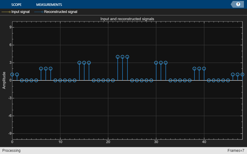
入力信号を再構成後の出力と比較する。
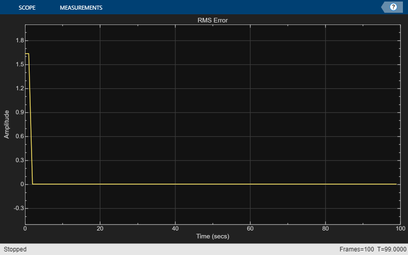
入力信号と最高正誤の出力の間の誤差を測定する。
システム全体の振幅応答をプロットする。
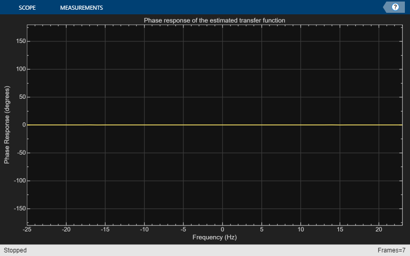
システム全体の位相応答をプロットする。
% Scope to compare input signal with reconstructed output
sigcompare = dsp.ArrayPlot('NumInputPorts', 2, 'ShowLegend', true,...
    'Title', 'Input and reconstructed signals',...
    'ChannelNames',{'Input signal','Reconstructed signal'});

% Scope to plot the RMS error between the input and reconstructed signals
errorPlot = timescope('Title', 'RMS Error', 'SampleRate', 1, ...
    'TimeUnits', 'seconds', 'YLimits', [-0.5 2],...
    'TimeSpanSource', 'property','TimeSpan',100,...
    'TimeSpanOverrunAction','scroll');

% To calculate the transfer function of the cascade of Analysis and
% Synthesis subband filters
tfestimate = dsp.TransferFunctionEstimator('FrequencyRange','centered',...
    'SpectralAverages', 50);
% Scope to plot the magnitude response of the estimated transfer function
magplot = dsp.ArrayPlot('PlotType','Line', ...
    'YLabel', 'Magnitude Response (dB)',...
    'Title','Magnitude response of the estimated transfer function',...
    'XOffset',-25, 'XLabel','Frequency (Hz)',...
    'YLimits',[-5 5]);
% Scope to plot the phase response of the estimated transfer function
phaseplot = dsp.ArrayPlot('PlotType','Line', ...
    'YLabel', 'Phase Response (degrees)',...
    'Title','Phase response of the estimated transfer function',...
    'XOffset',-25, 'XLabel','Frequency (Hz)',...
    'YLimits',[-180 180]);
完全再構成のシミュレーション
入力信号をサブバンド フィルターに渡し、出力を再構成します。スコープに結果をプロットします。
for i = 1:100
    % Use the same signal as input in each iteration.
    input = sigsource();
    % Analysis
    [hi, lo] = analysisFilter(input);
    % Synthesis
    reconstructed = synthFilter(hi, lo);

    % Compensate for the delay caused by the filters and compare the
    % signals. Since input signal is periodic, compare the current
    % frames of input and output signals.
    sigcompare(input(2:end), reconstructed(1:end-1));

    % Plot error between signals
    err = rms(input(2:end) - reconstructed(1:end-1));
    errorPlot(err);

    % Estimate transfer function of cascade
    Txy = tfestimate(input(2:end), reconstructed(1:end-1));
    magplot(20*log10(abs(Txy)));
    phaseplot(angle(Txy)*180/pi);
end
release(errorPlot);
release(magplot);

release(phaseplot);
完全再構成の出力分析
最初の 2 つのプロットから、2 チャネル フィルター バンクによって元の信号 x[n] が完全に再構成されたことがわかります。2 番目のプロットの初期の誤差はフィルターの遅延によるものです。3 番目および 4 番目のプロットは、システム全体の振幅応答が 0 dB、位相応答が 0° であり、その結果信号の周波数特性が保存されることを示しています。
関連するトピック
You can also select a web site from the following list:
Americas
- América Latina (Español)
- Canada (English)
- United States (English)
Europe
- Belgium (English)
- Denmark (English)
- Deutschland (Deutsch)
- España (Español)
- Finland (English)
- France (Français)
- Ireland (English)
- Italia (Italiano)
- Luxembourg (English)
- Netherlands (English)
- Norway (English)
- Österreich (Deutsch)
- Portugal (English)
- Sweden (English)
- Switzerland
- United Kingdom (English)